第四章 第二部分：机器视觉-图像分类

1.机器视觉的应用。

比如医疗领域，图像分类典型算法介绍
实操练习：数据预处理、搭建模型、调整参数。
学习深度学习的卷积神经网络。
狗与猫的分类、人与马的分类、手写体的分类

2.训练狗猫识别的卷积神经网络代码实现：

对狗和猫两种数据进行区分。

#调用程序里面常用的一些库，
import os	#os是文件操作的库
import zipfile 	#zip file主要是文件解压相关的一些库
import random	#random就是随机数发生器的库
import tensorflow as tf	#调用tensorflow深度学习的网络模型
from tensorflow.keras.optimizers import RMSprop #RMSPROP深度学习的优化算法
from tensorflow.keras.preprocessing.image import ImageDataGenerator #图进行预处理时调用ImageDataFenerator函数
from shutil import copyfile	#copyfile是对文件进行复制的一些库

# If the URL doesn't work, visit https://www.microsoft.com/en-us/download/confirmation.aspx?id=54765
# And right click on the 'Download Manually' link to get a new URL to the dataset。下载训练集链接，把文件存到tmp中。

# Note: This is a very large dataset and will take time to download
#wget命令linux进行下载，但是windows操作系统只需要用链接进行下载
#!wget --no-check-certificate \
#    "https://download.microsoft.com/download/3/E/1/3E1C3F21-ECDB-4869-8368-6DEBA77B919F/kagglecatsanddogs_3367a.zip" \
#    -O "/tmp/cats-and-dogs.zip"

#数据准备
local_zip = '/tmp/cats-and-dogs.zip'	
zip_ref   = zipfile.ZipFile(local_zip, 'r')	#调用ZipFile函数进行解压数据集
zip_ref.extractall('/tmp')	#解压到tmp文件中
zip_ref.close()

print(len(os.listdir('/tmp/PetImages/Cat/')))	#os.listdir方法查看tmp中文件，len函数表示文件的个数
print(len(os.listdir('/tmp/PetImages/Dog/')))

# Expected Output:
# 12501
# 12501

#把狗猫的数据分开，狗的数据放在testing文件夹里，
#mkdir创建文件目录，创建狗猫的测试数据和训练数据。
try:
    os.mkdir('/tmp/cats-v-dogs')
    os.mkdir('/tmp/cats-v-dogs/training')
    os.mkdir('/tmp/cats-v-dogs/testing')
    os.mkdir('/tmp/cats-v-dogs/training/cats')
    os.mkdir('/tmp/cats-v-dogs/training/dogs')
    os.mkdir('/tmp/cats-v-dogs/testing/cats')
    os.mkdir('/tmp/cats-v-dogs/testing/dogs')
except OSError:
    pass

#把解压的数据进行分割，分割成训练集和测试集。
import os
import shutil
#定义一个函数，split_data分割数据，把解压后的样本集，那把它切分成训练集training和testing sample。随机划分读进来。
def split_data(SOURCE, TRAINING, TESTING, SPLIT_SIZE):#split_size是切分的尺寸
    files = []
    for filename in os.listdir(SOURCE):#把样本集解压的文件一个个读出来放到file文件加里。
        file = SOURCE + filename
        if os.path.getsize(file) > 0:#判断文件大小，>0，把文件名读进去，追加到我们列表中。有效的图片
            files.append(filename)
        else:#如果不是，则报文件大小为0
            print(filename + " is zero length, so ignoring.")

    training_length = int(len(files) * SPLIT_SIZE)#读进来以后会调用split_size(0函数，如果这个函数参数是0.9,则是抽出90%的比例，把它划分到训练集里面进行训练。
    testing_length = int(len(files) - training_length)#测试样本就是总的样本文件减去刚抽出的测试样本集。
    shuffled_set = random.sample(files, len(files))#打乱文件顺序，random进行随机采样。
    training_set = shuffled_set[0:training_length]#训练样本集变成打乱以后样本集
    testing_set = shuffled_set[-testing_length:]#剩下的做为测试样本集。

    for filename in training_set:#读取训练样本集的
        this_file = SOURCE + filename#source是原来存放猫狗数据的原路径，加上文件名，就是要读的文件的路径。
        destination = TRAINING + filename
        copyfile(this_file, destination)#copyfile的命令可以把它读进来，读到训练样本集中，读到以后放到destination。实际上就是训练样本集一个个读进来，读进来读到training_length的长度。

    for filename in testing_set:#读取测试样本集的文件
        this_file = SOURCE + filename
        destination = TESTING + filename
        copyfile(this_file, destination)

#把训练样本、测试样本放在training这个子目录下。
CAT_SOURCE_DIR = "/tmp/PetImages/Cat/"#猫的数据
TRAINING_CATS_DIR = "/tmp/cats-v-dogs/training/cats/"#猫的训练样本集
TESTING_CATS_DIR = "/tmp/cats-v-dogs/testing/cats/"#猫的测试样本集
DOG_SOURCE_DIR = "/tmp/PetImages/Dog/"#狗的数据
TRAINING_DOGS_DIR = "/tmp/cats-v-dogs/training/dogs/"
TESTING_DOGS_DIR = "/tmp/cats-v-dogs/testing/dogs/"
#creat_dir命令产生路径，实际上就是前面样本集的路径，通过file_dir命令。
def create_dir(file_dir):
    if os.path.exists(file_dir):	#如果文件路径存在，打印true
        print('true')
        #os.rmdir(file_dir)
        shutil.rmtree(file_dir)#删除再建立
        os.makedirs(file_dir)
    else:
        os.makedirs(file_dir)
#调用函数，通过函数名（参数），生成四个子目录
create_dir(TRAINING_CATS_DIR)
create_dir(TESTING_CATS_DIR)
create_dir(TRAINING_DOGS_DIR)
create_dir(TESTING_CATS_DIR)
#把解压后的数据集进行切分，分割比例定为0.9
split_size = .9
#调用split_data函数，主要功能把猫的数据和狗的数据分别地把它切分层训练集和测试集，切分比例90%，就是训练样本90%,测试样本10%
split_data(CAT_SOURCE_DIR, TRAINING_CATS_DIR, TESTING_CATS_DIR, split_size)
split_data(DOG_SOURCE_DIR, TRAINING_DOGS_DIR, TESTING_DOGS_DIR, split_size)

# Expected output
# 666.jpg is zero length, so ignoring
# 11702.jpg is zero length, so ignoring

#打印样本进行切分以后每个文件夹文件的个数
print(len(os.listdir('/tmp/cats-v-dogs/training/cats/')))
print(len(os.listdir('/tmp/cats-v-dogs/training/dogs/')))
print(len(os.listdir('/tmp/cats-v-dogs/testing/cats/')))
print(len(os.listdir('/tmp/cats-v-dogs/testing/dogs/')))

# Expected output:
# 11250
# 11250
# 1250
# 1250

#搭建卷积网络，进行训练。调用了keras库中的model，三对卷积最大池化，
#参数16，32，64，512，1表示通道，随着隐层的加深，通道数量逐步增加。
model = tf.keras.models.Sequential([#sequential表示每一行表示一层，层与层之间都是顺序相连。
    tf.keras.layers.Conv2D(16, (3, 3), activation='relu', input_shape=(150, 150, 3)),#(3,3)表示卷积层的大小，relu是激活函数。输入层的输出就是150*150像素的三个通道。
    tf.keras.layers.MaxPooling2D(2, 2),#输出层的神经元为一个神经元，二分类问题，要么是狗要么是猫。
    tf.keras.layers.Conv2D(32, (3, 3), activation='relu'),
    tf.keras.layers.MaxPooling2D(2, 2),
    tf.keras.layers.Conv2D(64, (3, 3), activation='relu'),
    tf.keras.layers.MaxPooling2D(2, 2),
    tf.keras.layers.Flatten(),#第三对最大池化层flatten拉直。
    tf.keras.layers.Dense(512, activation='relu'),#接一个全链接的隐层，用的relu函数
    tf.keras.layers.Dense(1, activation='sigmoid')#然后再接到输出层，用到sigmoid函数
])

model.compile(optimizer=RMSprop(lr=0.001), loss='binary_crossentropy', metrics=['acc'])#学习步长是0.001，在梯度下降法训练网络过程中使用RMSprop修改学习步长。函数的损失函数用了二元交叉熵，网路性能的度量使用准确度。

#对数据进行预处理，ImageDataGenerator函数做规划，
TRAINING_DIR = "/tmp/cats-v-dogs/training/"
train_datagen = ImageDataGenerator(rescale=1.0/255.)#输入到输入层进行规划1/255，每个像素的编码都可以装成0~1之间的数值。
train_generator = train_datagen.flow_from_directory(TRAINING_DIR,
                                                    batch_size=100,#是epochs要循环的轮次
                                                    class_mode='binary',
                                                    target_size=(150, 150))
#对测试样本集做规划。
VALIDATION_DIR = "/tmp/cats-v-dogs/testing/"
validation_datagen = ImageDataGenerator(rescale=1.0/255.)
validation_generator = validation_datagen.flow_from_directory(VALIDATION_DIR,
batch_size=100,
class_mode='binary',
target_size=(150, 150))

# Expected Output:
# Found 22498 images belonging to 2 classes.
# Found 2500 images belonging to 2 classes.

#对网络进行训练，调用了model对象的fit_generator，fit就是拟合
# Note that this may take some time.
history = model.fit_generator(train_generator,
                              epochs=2,#说明拟合两轮，一轮就是所有的样本都要参加梯度下降，一批是对其中的100个样本进行训练。
                              verbose=1,#记录每次训练的日志
                              validation_data=validation_generator)

#查看训练结果，分析日志，
%matplotlib inline

import matplotlib.image  as mpimg
import matplotlib.pyplot as plt

#-----------------------------------------------------------
# Retrieve a list of list results on training and test data
# sets for each training epoch
#-----------------------------------------------------------
#从日志中得到训练样本的准确度、测试样本的准确度以及损失函数
acc=history.history['acc']
val_acc=history.history['val_acc']
#loss就是从history把损失函数也计算出来，包括训练样本的损失函数和测试样本的损失函数。
loss=history.history['loss']
val_loss=history.history['val_loss']

epochs=range(len(acc)) # Get number of epochs

#------------------------------------------------
# Plot training and validation accuracy per epoch
#------------------------------------------------
#输出成一个散点图，调用matplotlib中的plot,横坐标是epochs，，纵坐标是训练精度，两条线，输出两个图，分别值准确度和loss,红线是训练样本，蓝线是测试样本。
plt.plot(epochs, acc, 'r', "Training Accuracy")
plt.plot(epochs, val_acc, 'b', "Validation Accuracy")
plt.title('Training and validation accuracy')
plt.figure()

#------------------------------------------------
# Plot training and validation loss per epoch
#------------------------------------------------
plt.plot(epochs, loss, 'r', "Training Loss")
plt.plot(epochs, val_loss, 'b', "Validation Loss")
plt.figure()


# Desired output. Charts with training and validation metrics. No crash :)

# Here's a codeblock just for fun. You should be able to upload an image here 
# and have it classified without crashing
#功能：输入新的图片进行预处理以后输入到训练好的网络，网络就会预测图片到底是狗还是猫，
import numpy as np
from google.colab import files
from keras.preprocessing import image

uploaded = files.upload()

for fn in uploaded.keys():
 
  # predicting images
  path = '/content/' + fn
  img = image.load_img(path, target_size=(150, 150))#加载文件名路径，图像大小为150*150像素
  x = image.img_to_array(img)#把编码列表转成数组的形式
  x = np.expand_dims(x, axis=0)#把多维数组通过expand_dims命令拉直成相应的向量。

  images = np.vstack([x])#vstack按照水平方向把expand_dim各个通道的数据连起来构成一个长向量。
  classes = model.predict(images, batch_size=10)#模型预测运行输出对应的类别。
  print(classes[0])
  if classes[0]>0.5:#类别的可能性，输出层>0.5表示图片是狗，否则是猫
    print(fn + " is a dog")
  else:
    print(fn + " is a cat")

人马分类案例：

下载链接：https://storage.googleapis.com/laurencemoroney-blog.appspot.com/horse-or-human.zip
下面的python代码将使用OS库来调用文件系统，并使用zipfile库来解压数据。

import os
import zipfile

local_zip = '/tmp/horse-or-human.zip'
zip_ref = zipfile.ZipFile(local_zip, 'r')
zip_ref.extractall('/tmp/horse-or-human')
zip_ref.close()

Zip文件的内容会被解压到目录/tmp/horse-or-human，而该目录下又分别包含horses和humans子目录。
简而言之：训练集就是用来告诉神经网络模型 “这就是马的样子”、"这就是人的样子 "等数据。
这里需要注意的是，我们并没有明确地将图像标注为马或人。如果还记得之前的手写数字例子，它的训练数据已经标注了 “这是一个1”，"这是一个7 "等等。 稍后，我们使用一个叫做ImageGenerator的类–用它从子目录中读取图像，并根据子目录的名称自动给图像贴上标签。所以，会有一个 "训练 "目录，其中包含一个 "马匹 "目录和一个 "人类 "目录。ImageGenerator将为你适当地标注图片，从而减少一个编码步骤。（不仅编程上更方便，而且可以避免一次性把所有训练数据载入内存，而导致内存不够等问题。）
让我们分别定义这些目录。

# Directory with our training horse pictures
train_horse_dir = os.path.join('/tmp/horse-or-human/horses')

# Directory with our training human pictures
train_human_dir = os.path.join('/tmp/horse-or-human/humans')#生成两个文件夹存储马和人的数据

现在，让我们看看 "马 "和 "人 "训练目录中的文件名是什么样的。

train_horse_names = os.listdir(train_horse_dir)
print(train_horse_names[:10])

train_human_names = os.listdir(train_human_dir)
print(train_human_names[:10])#从两个子文件读10个文件名

结果：
[‘horse39-1.png’, ‘horse47-6.png’, ‘horse12-1.png’, ‘horse23-7.png’, ‘horse11-0.png’, ‘horse50-8.png’, ‘horse38-5.png’, ‘horse42-3.png’, ‘horse29-5.png’, ‘horse36-6.png’]
[‘human09-00.png’, ‘human09-14.png’, ‘human11-11.png’, ‘human04-14.png’, ‘human14-14.png’, ‘human07-03.png’, ‘human06-04.png’, ‘human09-29.png’, ‘human08-03.png’, ‘human14-16.png’]

我们来看看目录中马和人的图片总数。
#统计训练样本集中马和人的图片总数。

print('total training horse images:', len(os.listdir(train_horse_dir)))
print('total training human images:', len(os.listdir(train_human_dir)))

结果：
total training horse images: 500
total training human images: 527

现在我们来看看几张图片，以便对它们的样子有个直观感受。首先，配置matplot参数。
#把马和人的数据显示出来

%matplotlib inline

import matplotlib.pyplot as plt
import matplotlib.image as mpimg
#显示4行4列，16个图片
# Parameters for our graph; we'll output images in a 4x4 configuration
nrows = 4
ncols = 4

# Index for iterating over images
pic_index = 0#定义图的索引

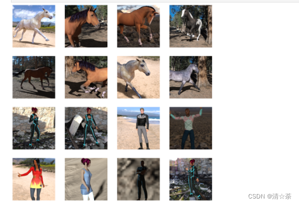
接下来，显示一批8张马和8张人的图片。每次重新运行单元格，都会看到一个新的批次（另外8张马和8张人）。定义图的尺寸

# Set up matplotlib fig, and size it to fit 4x4 pics
fig = plt.gcf()
fig.set_size_inches(ncols * 4, nrows * 4)

pic_index += 8	#图的索引加8
next_horse_pix = [os.path.join(train_horse_dir, fname) 
                for fname in train_horse_names[pic_index-8:pic_index]]#把马的名字读进来，读的是索引从马的子目录下是0~7的前八张图像，复制给前面的变量
next_human_pix = [os.path.join(train_human_dir, fname) 
                for fname in train_human_names[pic_index-8:pic_index]]

for i, img_path in enumerate(next_horse_pix+next_human_pix):#使用for循环把16张图片显示出来，使用了枚举方法
  # Set up subplot; subplot indices start at 1
  sp = plt.subplot(nrows, ncols, i + 1)#四行四类，i+1为图的位置
  sp.axis('Off') # Don't show axes (or gridlines)#图不显示坐标

  img = mpimg.imread(img_path)#imread表示把图读进来
  plt.imshow(img)

plt.show()

从零开始建立一个小型模型
让我们开始定义模型：
第一步是导入tensorflow

import tensorflow as tf

然后，像前面的例子一样添加卷积层，并将最终结果扁平化，以输送到全连接的层去。
最后我们添加全连接层。
需要注意的是，由于我们面对的是一个两类分类问题，即二类分类问题，所以我们会用sigmoid激活函数作为模型的最后一层，这样我们网络的输出将是一个介于0和1之间的有理数，即当前图像是1类（而不是0类）的概率。

model = tf.keras.models.Sequential([
    # Note the input shape is the desired size of the image 300x300 with 3 bytes color
    # This is the first convolution
    #
    tf.keras.layers.Conv2D(16, (3,3), activation='relu', input_shape=(150, 150, 3)),
    tf.keras.layers.MaxPooling2D(2, 2),
    # The second convolution
    tf.keras.layers.Conv2D(32, (3,3), activation='relu'),
    tf.keras.layers.MaxPooling2D(2,2),
    # The third convolution
    tf.keras.layers.Conv2D(64, (3,3), activation='relu'),
    tf.keras.layers.MaxPooling2D(2,2),
    # The fourth convolution
    tf.keras.layers.Conv2D(64, (3,3), activation='relu'),
    tf.keras.layers.MaxPooling2D(2,2),
    # The fifth convolution
    tf.keras.layers.Conv2D(64, (3,3), activation='relu'),
    tf.keras.layers.MaxPooling2D(2,2),
    # Flatten the results to feed into a DNN
    tf.keras.layers.Flatten(),
    # 512 neuron hidden layer
    tf.keras.layers.Dense(512, activation='relu'),
    # Only 1 output neuron. It will contain a value from 0-1 where 0 for 1 class ('horses') and 1 for the other ('humans')
    tf.keras.layers.Dense(1, activation='sigmoid')
])

调用model.summary()方法打印出神经元网络模型的结构信息

model.summary()

结果：

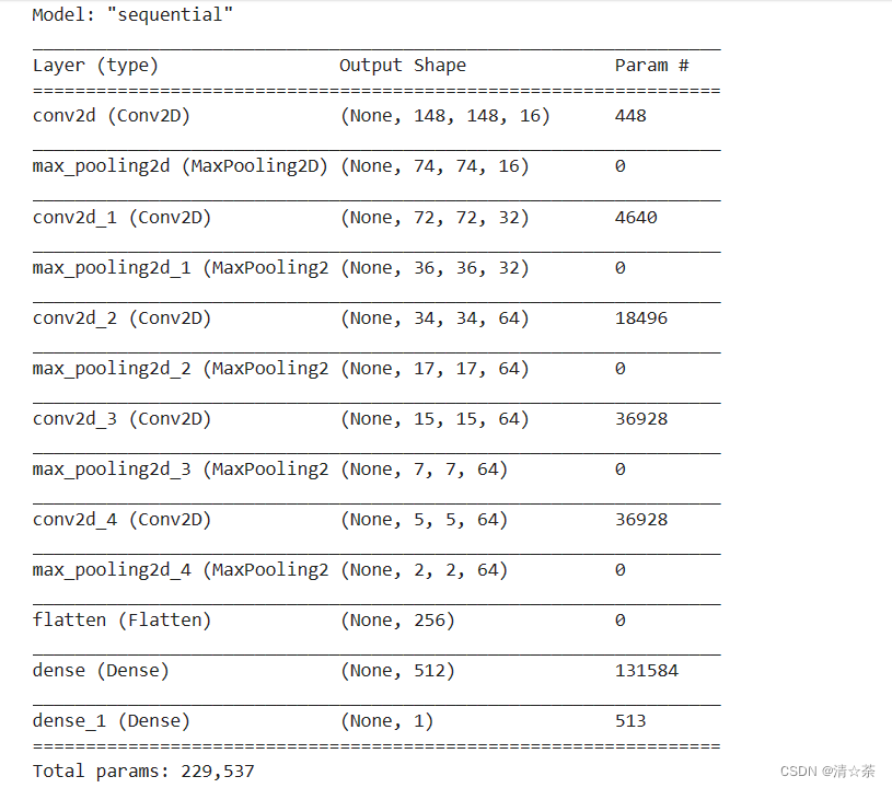
"输出形状 "一栏显示了特征图尺寸在每个层中是如何演变的。卷积层由于边框关系而使特征图的尺寸减小了一些，而每个池化层则将输出尺寸减半。
接下来，我们将配置模型训练的参数。我们将用 "binary_crossentropy（二元交叉熵）"衡量损失，因为这是一个二元分类问题，最终的激活函数是一个sigmoid。关于损失度量的复习，请参见机器学习速成班。我们将使用rmsprop作为优化器，学习率为0.001。在训练过程中，我们将希望监控分类精度。
NOTE：我们将使用学习率为0.001的rmsprop优化器。在这种情况下，使用RMSprop优化算法比随机梯度下降(SGD)更可取，因为RMSprop可以为我们自动调整学习率。(其他优化器，如Adam和Adagrad，也会在训练过程中自动调整学习率，在这里也同样有效。)

from tensorflow.keras.optimizers import RMSprop

model.compile(loss='binary_crossentropy',
              optimizer=RMSprop(lr=0.001),
              metrics=['acc'])

数据预处理
让我们设置训练数据生成器（ImageDataGenerator），它将读取源文件夹中的图片，将它们转换为float32多维数组，并将图像数据（连同它们的标签）反馈给神经元网络。总共需要两个生成器，有用于产生训练图像，一个用于产生验证图像。生成器将产生一批大小为300x300的图像及其标签（0或1）。
前面的课中我们已经知道如何对训练数据做归一化，进入神经网络的数据通常应该以某种方式进行归一化，以使其更容易被网络处理。在这个例子中，我们将通过将像素值归一化到[0, 1]范围内（最初所有的值都在[0, 255]范围内）来对图像进行预处理。
在Keras中，可以通过keras.preprocessing.image.ImageDataGenerator类使用rescale参数来实现归一化。通过ImageDataGenerator类的.flow(data, labels)或.flow_from_directory(directory)，可以创建生成器。然后，这些生成器可以作为输入Keras方法的参数，如fit_generator、evaluate_generator和predict_generator都可接收生成器实例为参数。

from tensorflow.keras.preprocessing.image import ImageDataGenerator

# All images will be rescaled by 1./255
train_datagen = ImageDataGenerator(rescale=1/255)

# Flow training images in batches of 128 using train_datagen generator
train_generator = train_datagen.flow_from_directory(
        '/tmp/horse-or-human/',  # This is the source directory for training images
        target_size=(150, 150),  # All images will be resized to 150x150
        batch_size=32, #128
        # Since we use binary_crossentropy loss, we need binary labels
        class_mode='binary')

结果：Found 1027 images belonging to 2 classes.

#训练
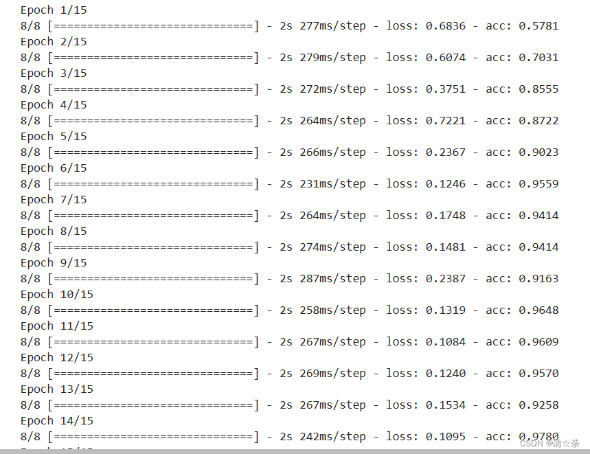
让我们训练15个epochs–这可能需要几分钟的时间完成运行。
请注意每次训练后的数值。
损失和准确率是训练进展的重要指标。模型对训练数据的类别进行预测，然后根据已知标签进行评估，计算准确率。准确率是指正确预测的比例。

history = model.fit(
      train_generator,
      steps_per_epoch=8,  
      epochs=15,
      verbose=1)

训练结果：

运行模型

接下来，看看使用模型进行实际预测。这段代码将允许你从文件系统中选择1个或多个文件，然后它将上传它们，并通过模型判断给出图像是马还是人。

import numpy as np
from google.colab import files
from tensorflow.keras.preprocessing import image

uploaded = files.upload()

for fn in uploaded.keys():
 
  # predicting images
  path = '/content/' + fn
  img = image.load_img(path, target_size=(300, 300))
  x = image.img_to_array(img)#把编码转成数组
  x = np.expand_dims(x, axis=0)#水平方向转成向量

  images = np.vstack([x])#把三个向量连起来，展成一个
  classes = model.predict(images, batch_size=10)
  print(classes[0])
  if classes[0]>0.5:
    print(fn + " is a human")
  else:
    print(fn + " is a horse")
 

报错：
ModuleNotFoundError: No module named ‘google-cloab’
解决方法：进入Anaconda Prompt中先输入conda activate textenv切换环境。
然后再下载：conda install -c conda-forge google-colab
如果执行出现C:\ProgramData\Anaconda3\envs\textenv\Lib\site-packages\google\colab__init__文件报错，直接把报错行代码注释掉。

将中间层的输出可视化
要想了解 convnet（卷积层）学到了什么样的特征，一个有趣的办法是将模型每个卷积层的输出当作图像可视化。
让我们从训练集中随机选取一张图像，然后将每一层的输出排列在一行里，生成一个汇总图。行中的每张图像都是一个特定过滤器输出的特征。每次运行下面这个单元的代码，就会随机显示一张图像的中间输出结果。

import numpy as np
import random
from tensorflow.keras.preprocessing.image import img_to_array, load_img

# Let's define a new Model that will take an image as input, and will output
# intermediate representations for all layers in the previous model after
# the first.
successive_outputs = [layer.output for layer in model.layers[1:]]
#visualization_model = Model(img_input, successive_outputs)
visualization_model = tf.keras.models.Model(inputs = model.input, outputs = successive_outputs)
# Let's prepare a random input image from the training set.
horse_img_files = [os.path.join(train_horse_dir, f) for f in train_horse_names]
human_img_files = [os.path.join(train_human_dir, f) for f in train_human_names]#从训练集中随机挑选数据
img_path = random.choice(horse_img_files + human_img_files)

img = load_img(img_path, target_size=(300, 300))  # this is a PIL image
x = img_to_array(img)  # Numpy array with shape (150, 150, 3)#数据转成数组
x = x.reshape((1,) + x.shape)  # Numpy array with shape (1, 150, 150, 3)

# Rescale by 1/255
x /= 255

# Let's run our image through our network, thus obtaining all
# intermediate representations for this image.
successive_feature_maps = visualization_model.predict(x)

# These are the names of the layers, so can have them as part of our plot
layer_names = [layer.name for layer in model.layers]

# Now let's display our representations
for layer_name, feature_map in zip(layer_names, successive_feature_maps):
  if len(feature_map.shape) == 4:
    # Just do this for the conv / maxpool layers, not the fully-connected layers
    n_features = feature_map.shape[-1]  # number of features in feature map
    # The feature map has shape (1, size, size, n_features)
    size = feature_map.shape[1]
    # We will tile our images in this matrix
    display_grid = np.zeros((size, size * n_features))
    for i in range(n_features):
      # Postprocess the feature to make it visually palatable
      x = feature_map[0, :, :, i]
      x -= x.mean()
      x /= x.std()
      x *= 64
      x += 128
      x = np.clip(x, 0, 255).astype('uint8')
      # We'll tile each filter into this big horizontal grid
      display_grid[:, i * size : (i + 1) * size] = x
    # Display the grid
    scale = 20. / n_features
    plt.figure(figsize=(scale * n_features, scale))
    plt.title(layer_name)
    plt.grid(False)
    plt.imshow(display_grid, aspect='auto', cmap='viridis')

从上面结果可以看出，图像每通过模型的一层，像素特征变得越来越抽象和紧凑。逐渐地，表征开始突出网络所关注的内容，它们显示出越来越少的像素被 “激活”；大多数被设置为零。这就是所谓的 “稀疏性”。表征稀疏性是深度学习的一个关键特征。

这些表征携带的图像原始像素的信息越来越少，但关于图像类别的信息却越来越精细。你可以把一个convnet（或一般的深度网络）看作是一个信息提炼管道。

清理：
运行以下单元格可以终止内核并释放内存资源。当计算资源不够时需要进行释放。

import os, signal
os.kill(os.getpid(), signal.SIGKILL)

调参
构造神经元网络模型时，一定会考虑需要几个卷积层？过滤器应该几个？全连接层需要几个神经元？

最先想到的肯定是手动修改那些参数，然后观察训练的效果（损失和准确度），从而判断参数的设置是否合理。但是那样很繁琐，因为参数组合会有很多，训练时间很长。再进一步，可以手动编写一些循环，通过遍历来搜索合适的参数。但是最好利用专门的框架来搜索参数，不太容易出错，效果也比前两种方法更好。

Kerastuner就是一个可以自动搜索模型训练参数的库。它的基本思路是在需要调整参数的地方插入一个特殊的对象（可指定参数范围），然后调用类似训练那样的search方法即可。

接下来首先准备训练数据和需要加载的库。

import os
from tensorflow.keras.preprocessing.image import ImageDataGenerator
from tensorflow.keras.optimizers import RMSprop
train_datagen = ImageDataGenerator(rescale=1/255)
validation_datagen = ImageDataGenerator(rescale=1/255)
train_generator = train_datagen.flow_from_directory('/tmp/horse-or-human/',  
        target_size=(150, 150),batch_size=32,class_mode='binary')
validation_generator = validation_datagen.flow_from_directory('/tmp/validation-horse-or-human/',  
        target_size=(150, 150), batch_size=32,class_mode='binary')
from kerastuner.tuners import Hyperband
from kerastuner.engine.hyperparameters import HyperParameters
import tensorflow as tf

接着创建HyperParameters对象，然后在模型中插入Choice、Int等调参用的对象。

hp=HyperParameters()
def build_model(hp):
    model = tf.keras.models.Sequential()        
    model.add(tf.keras.layers.Conv2D(hp.Choice('num_filters_top_layer',values=[16,64],default=16), (3,3), 
                                     activation='relu', input_shape=(150, 150, 3)))
    model.add(tf.keras.layers.MaxPooling2D(2, 2))
    for i in range(hp.Int("num_conv_layers",1,3)):
        model.add(tf.keras.layers.Conv2D(hp.Choice(f'num_filters_layer{i}',values=[16,64],default=16), (3,3), activation='relu'))
        model.add(tf.keras.layers.MaxPooling2D(2,2))
    model.add(tf.keras.layers.Flatten())
    model.add(tf.keras.layers.Dense(hp.Int("hidden_units",128,512,step=32), activation='relu'))
    model.add(tf.keras.layers.Dense(1, activation='sigmoid'))
    model.compile(loss='binary_crossentropy',optimizer=RMSprop(lr=0.001),metrics=['acc'])
    return model

然后创建Hyperband对象，这是Kerastuner支持的四种方法的其中一种，其优点是能较四童话第查找参数。具体资料可以到Kerastuner的网站获取。

最后调用search方法。

tuner=Hyperband(
    build_model,
    objective='val_acc',
    max_epochs=10,
    directory='horse_human_params',
    hyperparameters=hp,
    project_name='my_horse_human_project'
)
tuner.search(train_generator,epochs=10,validation_data=validation_generator)

搜索到最优参数后，可以通过下面的程序，用tuner对象提取最优参数构建神经元网络模型。并调用summary方法观察优化后的网络结构。

best_hps=tuner.get_best_hyperparameters(1)[0]
print(best_hps.values)
model=tuner.hypermodel.build(best_hps)
model.summary()

手写体识别案例：

import csv
import numpy as np
import tensorflow as tf
from tensorflow.keras.preprocessing.image import ImageDataGenerator

def get_data(filename):
    with open(filename) as training_file:
        csv_reader = csv.reader(training_file, delimiter=',')
        first_line = True
        temp_images = []
        temp_labels = []
        for row in csv_reader:
            if first_line:
                # print("Ignoring first line")
                first_line = False
            else:
                temp_labels.append(row[0])
                image_data = row[1:785]
                image_data_as_array = np.array_split(image_data, 28)
                temp_images.append(image_data_as_array)
        images = np.array(temp_images).astype('float')
        labels = np.array(temp_labels).astype('float')
    return images, labels


training_images, training_labels = get_data('sign_mnist_train.csv')
testing_images, testing_labels = get_data('sign_mnist_test.csv')

print(training_images.shape)
print(training_labels.shape)
print(testing_images.shape)
print(testing_labels.shape)

(27455, 28, 28)
(27455,)
(7172, 28, 28)
(7172,)

training_images = np.expand_dims(training_images, axis=3)
testing_images = np.expand_dims(testing_images, axis=3)

train_datagen = ImageDataGenerator(
    rescale=1. / 255,
    rotation_range=40,
    width_shift_range=0.2,
    height_shift_range=0.2,
    shear_range=0.2,
    zoom_range=0.2,
    horizontal_flip=True,
    fill_mode='nearest')

validation_datagen = ImageDataGenerator(
    rescale=1. / 255)

print(training_images.shape)
print(testing_images.shape)

(27455, 28, 28, 1)
(7172, 28, 28, 1)

model = tf.keras.models.Sequential([
    tf.keras.layers.Conv2D(64, (3, 3), activation='relu', input_shape=(28, 28, 1)),
    tf.keras.layers.MaxPooling2D(2, 2),
    tf.keras.layers.Conv2D(64, (3, 3), activation='relu'),
    tf.keras.layers.MaxPooling2D(2, 2),
    tf.keras.layers.Flatten(),
    tf.keras.layers.Dense(128, activation=tf.nn.relu),
    tf.keras.layers.Dense(26, activation=tf.nn.softmax)])

# Before modification
# model.compile(optimizer = tf.train.AdamOptimizer(),
#              loss = 'sparse_categorical_crossentropy',
#              metrics=['accuracy'])
#

# After modification
model.compile(optimizer = tf.optimizers.Adam(),
              loss = 'sparse_categorical_crossentropy',
              metrics=['accuracy'])

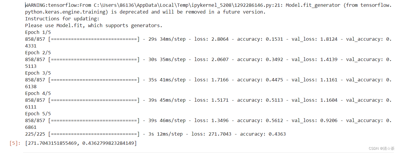
history = model.fit_generator(train_datagen.flow(training_images, training_labels, batch_size=32),
                              steps_per_epoch=len(training_images) / 32,
                              epochs=5,
                              validation_data=validation_datagen.flow(testing_images, testing_labels, batch_size=32),
                              validation_steps=len(testing_images) / 32)

model.evaluate(testing_images, testing_labels)

import matplotlib.pyplot as plt
acc = history.history['acc']
val_acc = history.history['val_acc']
loss = history.history['loss']
val_loss = history.history['val_loss']

epochs = range(len(acc))

plt.plot(epochs, acc, 'r', label='Training accuracy')
plt.plot(epochs, val_acc, 'b', label='Validation accuracy')
plt.title('Training and validation accuracy')
plt.legend()
plt.figure()

plt.plot(epochs, loss, 'r', label='Training Loss')
plt.plot(epochs, val_loss, 'b', label='Validation Loss')
plt.title('Training and validation loss')
plt.legend()

plt.show()