自适应雷达检测中纹理相关复合高斯矢量的协方差矩阵估计（Matlab代码实现）-CSDN博客

本文链接：https://blog.csdn.net/qq_46009436/article/details/143354980

💥💥💞💞欢迎来到本博客❤️❤️💥💥

🏆博主优势：🌞🌞🌞博客内容尽量做到思维缜密，逻辑清晰，为了方便读者。

⛳️座右铭：行百里者，半于九十。

📋📋📋本文目录如下：🎁🎁🎁

目录

⛳️赠与读者

💥1 概述

📚2 运行结果

🎉3 参考文献

🌈4 Matlab代码实现

⛳️赠与读者

👨‍💻做科研，涉及到一个深在的思想系统，需要科研者逻辑缜密，踏实认真，但是不能只是努力，很多时候借力比努力更重要，然后还要有仰望星空的创新点和启发点。当哲学课上老师问你什么是科学，什么是电的时候，不要觉得这些问题搞笑。哲学是科学之母，哲学就是追究终极问题，寻找那些不言自明只有小孩子会问的但是你却回答不出来的问题。建议读者按目录次序逐一浏览，免得骤然跌入幽暗的迷宫找不到来时的路，它不足为你揭示全部问题的答案，但若能让人胸中升起一朵朵疑云，也未尝不会酿成晚霞斑斓的别一番景致，万一它居然给你带来了一场精神世界的苦雨，那就借机洗刷一下原来存放在那儿的“躺平”上的尘埃吧。

或许，雨过云收，神驰的天地更清朗.......🔎🔎🔎

💥1 概述

摘要：
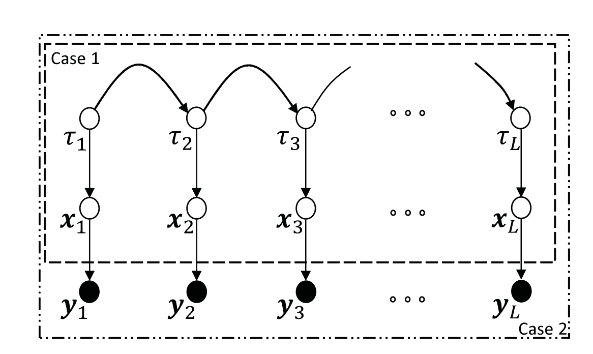
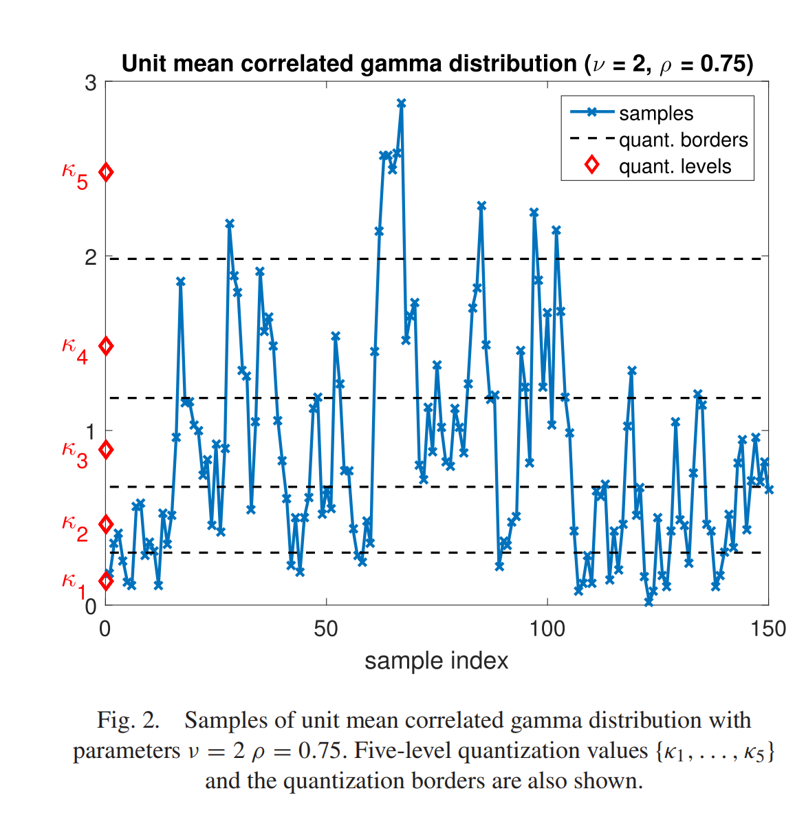
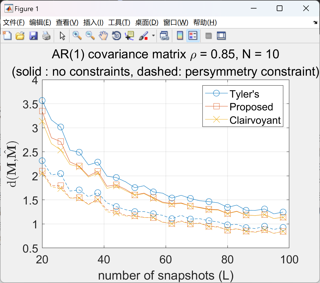
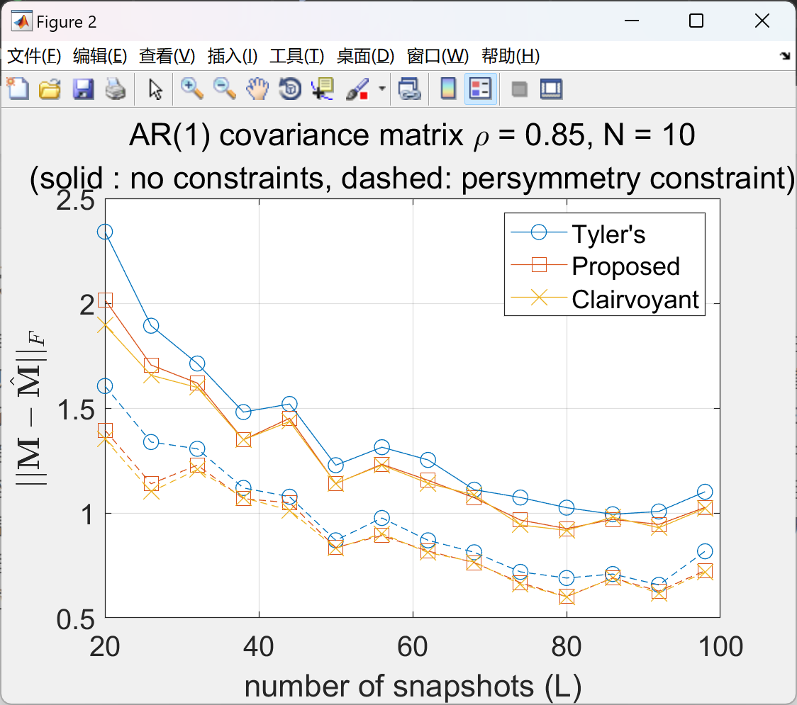
本文研究了具有纹理相关性的复合高斯向量（自适应雷达探测器的空间相关性）的协方差矩阵估计。纹理参数被视为隐藏的随机参数，其统计描述由马尔可夫链给出。链的状态表示纹理系数的值，过渡概率建立了纹理序列中的相关性。针对无噪声和有噪声快照，给出了基于期望最大化（EM）方法的协方差矩阵估计解决方案。对具有实际重要性的对称协方差矩阵的扩展得到了发展，并描述了可能扩展到其他结构化协方差矩阵的情况。数值结果表明，在协方差矩阵估计中利用空间相关性的好处可能是显著的，尤其是在次级数据中的快照总数较少的情况下。从应用的角度来看，所提出的模型非常适合海杂波中的自适应目标检测，实验观察到距离单元之间存在一些空间相关性。所建议的少量快照方法的性能改进在这个应用领域尤为重要。

Abstract:

In this article, covariance matrix estimation of compound-Gaussian vectors with texture-correlation (spatial correlation for the adaptive radar detectors) is examined. The texture parameters are treated as hidden random parameters whose statistical description is given by a Markov chain. States of the chain represent the value of texture coefficient and the transition probabilities establish the correlation in the texture sequence. An expectation–maximization (EM) method-based covariance matrix estimation solution is given for both noiseless and noisy snapshots. An extension to the practically important case of persymmetric covariance matrices is developed and possible extensions to other structured covariance matrices are described. The numerical results indicate that the benefit of utilizing spatial correlation in the covariance matrix estimation can be significant especially when the total number of snapshots in the secondary data is small. From applications viewpoint, the suggested model is well suited for the adaptive target detection in sea clutter, where some spatial correlation between range cells has been experimentally observed. The performance improvements of the suggested approach for small number of snapshots can be particularly important in this application area.

准确可靠（异常值鲁棒性）的问题从有限数量的数据中估计协方差矩阵快照在许多应用程序中至关重要。这个该问题通常针对联合高斯多变量（高斯向量）进行处理；但在某些应用中，例如杂波建模，快照矢量的总功率可以快照与快照之间波动显著，导致与标准模型的偏差。对于此类应用统计文献中的异常值稳健估计量，如作为Tyler的估计量[1]，归一化样本协方差矩阵[2]和Huber的M估计器[3]、[4]已被进行了深入的研究，包括一些特定应用的需求在设计过程中，如样本不足、低秩约束、已知矩阵结构、知识辅助操作[5]、[6]、[7]、[8]、[9]、[10]。常见的假设在这些研究中，快照的统计独立性是关键矢量。在这项研究中，我们研究了相关案例协方差矩阵估计和呈现的快照一种用于嘈杂/无噪声快照的多功能解决方案。案件对噪声相关快照的压缩具有实际意义机载/海基自适应雷达探测器本研究的主要动机。自适应雷达探测器旨在直接或间接估计干扰（杂波加噪声）协方差矩阵从一组称为次级数据集的快照中[11]，[12]。更具体地说，凯利测试[13]和自适应相干估计器（ACE）[14]间接估计了未知广义似然函数中的干扰协方差矩阵比率测试（GLRT）框架。这两种测试是相似的但它们的假设存在重要差异。凯利的测试假设原始数据的协方差矩阵，也称为受试细胞（CUT），与次级数据单元的协方差矩阵（同质环境假设）。ACE假设协方差次级数据单元的矩阵是相同的；但不同通过未知缩放从CUT协方差矩阵中提取因素（部分同质环假设），[11，第2.3节]。详细文章见第4部分。

📚2 运行结果

部分代码：

Lvec = 20:3:100; %number of snapshots
N = 10; %dimension of snapshot vector
MCnum = 25; %Increase MCnum to get more reliable estimates at the expense of time! (MCnum is set as 500 to generate Figure 4a in the text.)
iterEM = 50;

%%%
rho = 0.85; %AR(1) process parameter (correlation coef.)

%Markov Chain Parameters
stay_in_prob = 0.9;
theta_vec = [0.01 0.1 1 10 100];
num_states = length(theta_vec);
p0 = 1/num_states*ones(num_states,1); %Equally likely state
%p0 = zeros(num_states,1); p0(theta_vec==1) = 1-0.05; %Starts from CUT power level

%Clutter Cov. Mat.
Rc = toeplitz(rho.^(0:N-1)); %Note trace{Rc} = N
sqrtRc = sqrtm(Rc);

h = waitbar(0,'Please wait...'); ind_L = 0;
cflipud = @(x) conj(flipud(x));
Rdistmat = zeros(length(Lvec),MCnum,3); Frobdistmat = zeros(length(Lvec),MCnum,3);
meanRdistmat = zeros(length(Lvec),3); meanFrobdistmat = zeros(length(Lvec),3);

Rdistmat_persym = zeros(length(Lvec),MCnum,3); Frobdistmat_persym = zeros(length(Lvec),MCnum,3);
meanRdistmat_persym = zeros(length(Lvec),3); meanFrobdistmat_persym = zeros(length(Lvec),3);
for L = Lvec,
ind_L = ind_L + 1;

%Markov Chain Transition Probability
P = (1-stay_in_prob)/(num_states-1)*ones(num_states,num_states) + ...
(num_states*stay_in_prob - 1)/(num_states-1)*eye(num_states,num_states);

%%
for indMC = 1:MCnum,
%Generate data
state_seq = gen_markov_process(p0,P,L);
s = theta_vec(state_seq); %s is the unknown variance sequence
Xmat = sqrtRc*randn(N,L);
%r = bsxfun(@times,Xmat,sqrt(s)) + sqrt(sigma_v_sq/2)*(randn(Npulse,L) + 1i*randn(Npulse,L));
r = bsxfun(@times,Xmat,sqrt(s));


%Estimators
%Rini = 1/L*(r*r'); Rini = Rini/sum(diag(Rini))*N;
Rini = cov_mat_est_Tyler(r,eye(N),5);
[Rest,posterior_prob] = cov_mat_est3f_noiseless(r,P,p0,theta_vec,Rini,iterEM);
Rest_clair = (Xmat*Xmat')/L; %Noiseless clutter snapshopts at CUT power level
Rest_Tyler = cov_mat_est_Tyler(r,eye(N),20);

%Estimators (persymmetric)
Rini = cov_mat_est_Tyler(r,eye(N),5);
[Rest_persym,posterior_prob_persym] = cov_mat_est3f_noiseless(r,P,p0,theta_vec,Rini,iterEM,'persymmetric');
Rest_clair_persym = (Xmat*Xmat' + cflipud(Xmat)*cflipud(Xmat)')/2/L; %Noiseless clutter snapshopts at CUT power level
Rest_Tyler_persym = cov_mat_est_Tyler(r,eye(N),20,'persymmetric');

%Trace normalize matrices
trval = N;

🎉3 参考文献

文章中一些内容引自网络，会注明出处或引用为参考文献，难免有未尽之处，如有不妥，请随时联系删除。

[1]Ç. Candan and F. Pascal, "Covariance Matrix Estimation of Texture Correlated Compound-Gaussian Vectors for Adaptive Radar Detection," in IEEE Transactions on Aerospace and Electronic Systems, vol. 59, no. 3, pp. 3009-3020, June 2023