


记
第二章开始正式开始学习认识一个具体的项目案例(房地产区域定价)。
1.创建工作区
在创建工作区部分介绍了基本的环境配置和jupyter的使用,书中是在Linux或macOS上的bash shell中使用pip进行安装的,实际上如果和我一样使用Windows的话安装Anaconda后即可直接在开始栏中找到并自动打开jupyter notebook,需要注意的是网页使用过程中终端不要关闭。
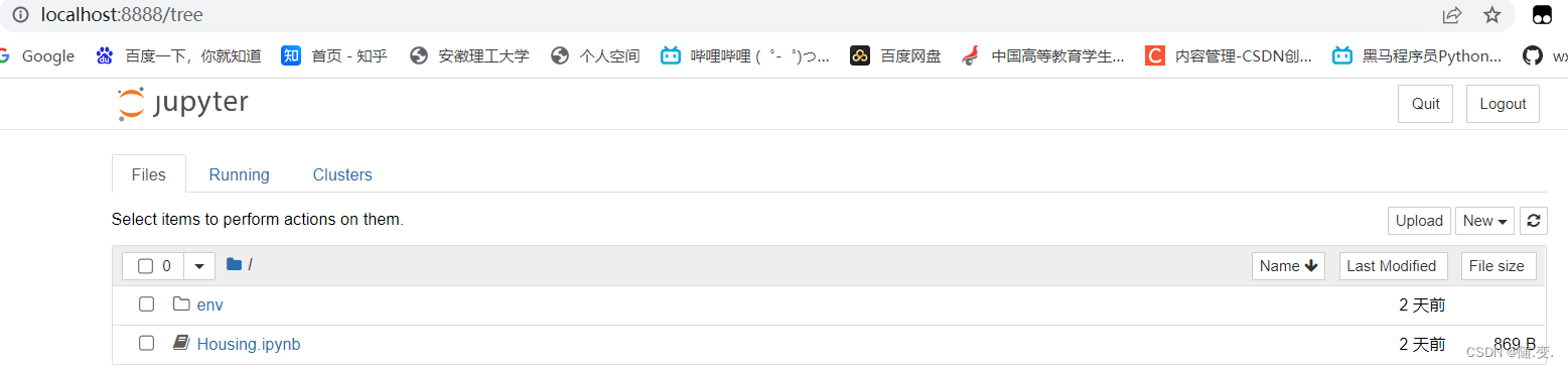
启动jupyter后会自动进入我们的工作网页,此时会发现和书中不一样,显示的是一个默认的目录(实际上就是主机用户的Administrator目录下内容),看起来不是很整洁,想要打开后直接进入我们自己创建的工作目录,只需要如下配置几步即可:
- 打开Anaconda Prompt,输入
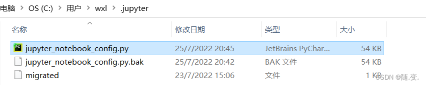
jupyter notebook --generate-config - 打开C:\Users\wxl\.jupyter\jupyter_notebook_config.py文件
- 自己另外创建一个工作目录,记下地址,打开2中的config文件,找到#c.NotebookApp.notebook_dir = ‘’,改为 c.NotebookApp.notebook_dir = ‘D:\ML\code_WXL’(引号内为自己创建的工作目录)
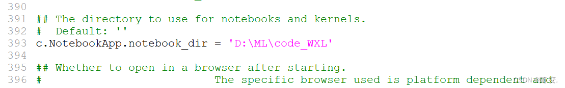
- 保存后再打开jupyter就可以直接进入自己创建的工作目录了
2.下 (加)载数据
接下来是利用Python编写一个自动获取网站数据集的脚本,值得注意的是,实际操作中会发现很多报错。
期初在pycharm中运行示例代码,后来发现总是会有很多奇怪的报错,很多是因为jupyter与pycharm的一些语法不同(例如显示图形),后来直接在jupyter上实验,效果不错也很方便。
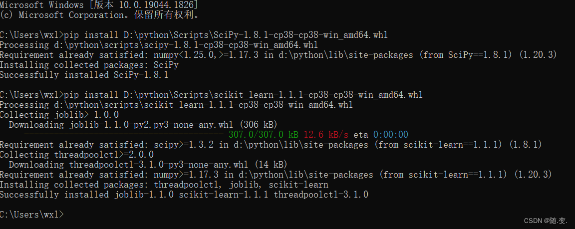
实验过程中首先是科学包的导入,直接在pycharm中安装包往往因为服务器延迟太高安装失败。
可以参考下面的安装方式成功导入。
sklearn库安装方法_林同学l的博客-CSDN博客_sklearn库怎么安装
科学包全部安装好后,除了书上给出的代码,还需要设置图形显示和导入科学包等等。代码如下:
# Python ≥3.5 is required
import sys
assert sys.version_info >= (3, 5)

# Scikit-Learn ≥0.20 is required
import sklearn
assert sklearn.__version__ >= "0.20"

# Common imports
import numpy as np
import os

# To plot pretty figures
%matplotlib inline
import matplotlib as mpl
import matplotlib.pyplot as plt
mpl.rc('axes', labelsize=14)
mpl.rc('xtick', labelsize=12)
mpl.rc('ytick', labelsize=12)

# Where to save the figures
PROJECT_ROOT_DIR = "."
CHAPTER_ID = "end_to_end_project"
IMAGES_PATH = os.path.join(PROJECT_ROOT_DIR, "images", CHAPTER_ID)
os.makedirs(IMAGES_PATH, exist_ok=True)

def save_fig(fig_id, tight_layout=True, fig_extension="png", resolution=300):
    path = os.path.join(IMAGES_PATH, fig_id + "." + fig_extension)
    print("Saving figure", fig_id)
    if tight_layout:
        plt.tight_layout()
    plt.savefig(path, format=fig_extension, dpi=resolution)

# Ignore useless warnings (see SciPy issue #5998)
import warnings
warnings.filterwarnings(action="ignore", message="^internal gelsd")
然后是从书作者的网站上获取数据集:(本人家中移动网络屡次报错超时<移动网真不行QAQ>,换电信网络后成功获取,但有明显延迟,最好挂VPN)
获取数据的函数:
import os
import tarfile
import urllib

DOWNLOAD_ROOT = "https://raw.githubusercontent.com/ageron/handson-ml2/master/"
HOUSING_PATH = os.path.join("datasets", "housing")
HOUSING_URL = DOWNLOAD_ROOT + "datasets/housing/housing.tgz"

def fetch_housing_data(housing_url=HOUSING_URL, housing_path=HOUSING_PATH):
    if not os.path.isdir(housing_path):
        os.makedirs(housing_path)
    tgz_path = os.path.join(housing_path, "housing.tgz")
    urllib.request.urlretrieve(housing_url, tgz_path)
    housing_tgz = tarfile.open(tgz_path)
    housing_tgz.extractall(path=housing_path)
    housing_tgz.close()
调用fetch_housing_data(),就会自动创建目录并解压数据集到该目录下。
加载数据:
import pandas as pd

def load_housing_data(housing_path=HOUSING_PATH):
    csv_path = os.path.join(housing_path, "housing.csv")
    return pd.read_csv(csv_path)

housing = load_housing_data()
housing.head()
调用后输出如下:

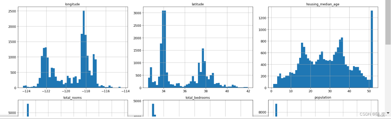
然后是调用一些方法查看了数据的属性。绘制了属性的直方图如下:
3.创建测试集
取20%的数据作为测试集,关键在于测试集不应发生改变,所以需要设置一个随机数生成器的种子 ,并对每个实例设置一个唯一的标识符。
实现方式如下:
from zlib import crc32

def test_set_check(identifier, test_ratio):
    return crc32(np.int64(identifier)) & 0xffffffff < test_ratio * 2**32

def split_train_test_by_id(data, test_ratio, id_column):
    ids = data[id_column]
    in_test_set = ids.apply(lambda id_: test_set_check(id_, test_ratio))
    return data.loc[~in_test_set], data.loc[in_test_set]

import hashlib

def test_set_check(identifier, test_ratio, hash=hashlib.md5):
    return hash(np.int64(identifier)).digest()[-1] < 256 * test_ratio

def test_set_check(identifier, test_ratio, hash=hashlib.md5):
    return bytearray(hash(np.int64(identifier)).digest())[-1] < 256 * test_ratio

housing_with_id = housing.reset_index()   # adds an `index` column
train_set, test_set = split_train_test_by_id(housing_with_id, 0.2, "index")

housing_with_id["id"] = housing["longitude"] * 1000 + housing["latitude"]
train_set, test_set = split_train_test_by_id(housing_with_id, 0.2, "id")

test_set.head()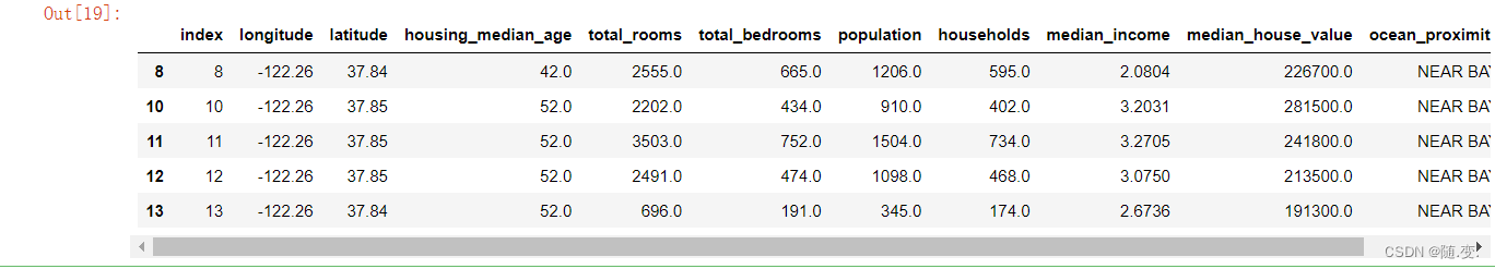
注意测试集采用分层抽样,否则测试结果会发生偏差。
4.数据探索
将经纬度可视化:
housing.plot(kind="scatter", x="longitude", y="latitude")
save_fig("bad_visualization_plot")
突出高密度区域:
housing.plot(kind="scatter", x="longitude", y="latitude", alpha=0.1)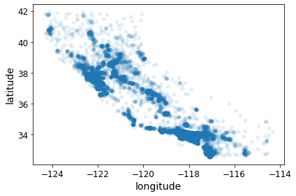
用圆圈大小表示人口数量,颜色代表价格:
housing.plot(kind="scatter", x="longitude", y="latitude", alpha=0.4,
    s=housing["population"]/100, label="population", figsize=(10,7),
    c="median_house_value", cmap=plt.get_cmap("jet"), colorbar=True,
    sharex=False)
plt.legend() 
查看各属性与房价中位数的相关性:
corr_matrix = housing.corr()
corr_matrix["median_house_value"].sort_values(ascending=False)
可见房价和收入成正相关,和维度成轻微负相关。
散布矩阵比较各数值属性(房价,收入,房间总数,住房年龄):
from pandas.plotting import scatter_matrix

attributes = ["median_house_value", "median_income", "total_rooms",
              "housing_median_age"]
scatter_matrix(housing[attributes], figsize=(12, 8))
单独查看收入和房价的关系:
housing.plot(kind="scatter", x="median_income", y="median_house_value",
             alpha=0.1)
plt.axis([0, 16, 0, 550000])
可以看出确实很明显成正相关,同时注意到有数条横线可能会影响后面的算法学习。
还可以将不同属性组合起来创建更有价值的属性来研究:
housing["rooms_per_household"] = housing["total_rooms"]/housing["households"]
housing["bedrooms_per_room"] = housing["total_bedrooms"]/housing["total_rooms"]
housing["population_per_household"]=housing["population"]/housing["households"]
corr_matrix = housing.corr()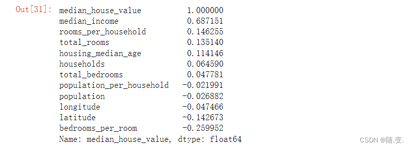
5.数据准备
首先复制一个干净的训练集:
housing = strat_train_set.drop("median_house_value", axis=1) # drop labels for training set
housing_labels = strat_train_set["median_house_value"].copy()
数据清理:将有缺失值的属性处理好 (自主填入或删除数据)
利用sklearn将中位数代替缺省值:
from sklearn.impute import SimpleImputer
imputer = SimpleImputer(strategy="median")
housing_num = housing.drop("ocean_proximity", axis=1)
imputer.fit(housing_num)
imputer.statistics_
housing_num.median().values
X = imputer.transform(housing_num)
housing_tr = pd.DataFrame(X, columns=housing_num.columns,
                          index=housing.index)
housing_tr.loc[sample_incomplete_rows.index.values]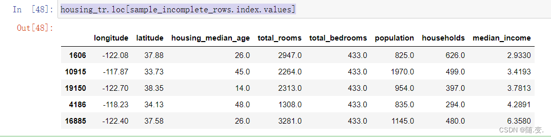
使用独热编码为文本属性编码:
from sklearn.preprocessing import OneHotEncoder

cat_encoder = OneHotEncoder()
housing_cat_1hot = cat_encoder.fit_transform(housing_cat)
housing_cat_1hot
自定义转换器
from sklearn.base import BaseEstimator, TransformerMixin

# column index
rooms_ix, bedrooms_ix, population_ix, households_ix = 3, 4, 5, 6

class CombinedAttributesAdder(BaseEstimator, TransformerMixin):
    def __init__(self, add_bedrooms_per_room=True): # no *args or **kargs
        self.add_bedrooms_per_room = add_bedrooms_per_room
    def fit(self, X, y=None):
        return self  # nothing else to do
    def transform(self, X):
        rooms_per_household = X[:, rooms_ix] / X[:, households_ix]
        population_per_household = X[:, population_ix] / X[:, households_ix]
        if self.add_bedrooms_per_room:
            bedrooms_per_room = X[:, bedrooms_ix] / X[:, rooms_ix]
            return np.c_[X, rooms_per_household, population_per_household,
                         bedrooms_per_room]
        else:
            return np.c_[X, rooms_per_household, population_per_household]

attr_adder = CombinedAttributesAdder(add_bedrooms_per_room=False)
housing_extra_attribs = attr_adder.transform(housing.values)
转换流水线(定义步骤序列)
from sklearn.pipeline import Pipeline
from sklearn.preprocessing import StandardScaler

num_pipeline = Pipeline([
        ('imputer', SimpleImputer(strategy="median")),
        ('attribs_adder', CombinedAttributesAdder()),
        ('std_scaler', StandardScaler()),
    ])

housing_num_tr = num_pipeline.fit_transform(housing_num)
处理列的转换器
from sklearn.compose import ColumnTransformer

num_attribs = list(housing_num)
cat_attribs = ["ocean_proximity"]

full_pipeline = ColumnTransformer([
        ("num", num_pipeline, num_attribs),
        ("cat", OneHotEncoder(), cat_attribs),
    ])

housing_prepared = full_pipeline.fit_transform(housing)
6.选择和训练模型
训练一个线性回归模型
from sklearn.linear_model import LinearRegression

lin_reg = LinearRegression()
lin_reg.fit(housing_prepared, housing_labels)
训练实例
some_data = housing.iloc[:5]
some_labels = housing_labels.iloc[:5]
some_data_prepared = full_pipeline.transform(some_data)

print("Predictions:", lin_reg.predict(some_data_prepared))
print("Labels:", list(some_labels))e_data_prepared))
测量回归模型的RMSE
from sklearn.metrics import mean_squared_error

housing_predictions = lin_reg.predict(housing_prepared)
lin_mse = mean_squared_error(housing_labels, housing_predictions)
lin_rmse = np.sqrt(lin_mse)
lin_rmse ![]()
可见模型欠拟合。
换一个模型:
from sklearn.tree import DecisionTreeRegressor

tree_reg = DecisionTreeRegressor(random_state=42)
tree_reg.fit(housing_prepared, housing_labels)
评估:
housing_predictions = tree_reg.predict(housing_prepared)
tree_mse = mean_squared_error(housing_labels, housing_predictions)
tree_rmse = np.sqrt(tree_mse)
tree_rmse![]()
可能过拟合了。
交叉验证:
from sklearn.model_selection import cross_val_score

scores = cross_val_score(tree_reg, housing_prepared, housing_labels,
                         scoring="neg_mean_squared_error", cv=10)
tree_rmse_scores = np.sqrt(-scores)

def display_scores(scores):
    print("Scores:", scores)
    print("Mean:", scores.mean())
    print("Standard deviation:", scores.std())

display_scores(tree_rmse_scores)
结果不好。换随机森林模型
from sklearn.ensemble import RandomForestRegressor

forest_reg = RandomForestRegressor(n_estimators=100, random_state=42)
forest_reg.fit(housing_prepared, housing_labels)
housing_predictions = forest_reg.predict(housing_prepared)
forest_mse = mean_squared_error(housing_labels, housing_predictions)
forest_rmse = np.sqrt(forest_mse)
forest_rmse

from sklearn.model_selection import cross_val_score

forest_scores = cross_val_score(forest_reg, housing_prepared, housing_labels,
                                scoring="neg_mean_squared_error", cv=10)
forest_rmse_scores = np.sqrt(-forest_scores)
display_scores(forest_rmse_scores)
结果要良好很多
7.调整模型
自动调整超参数
from sklearn.model_selection import GridSearchCV
param_grid = [
# try 12 (3×4) combinations of hyperparameters
{'n_estimators': [3, 10, 30], 'max_features': [2, 4, 6, 8]},
# then try 6 (2×3) combinations with bootstrap set as False
{'bootstrap': [False], 'n_estimators': [3, 10], 'max_features': [2, 3, 4]},
]
forest_reg = RandomForestRegressor(random_state=42)
# train across 5 folds, that's a total of (12+6)*5=90 rounds of training
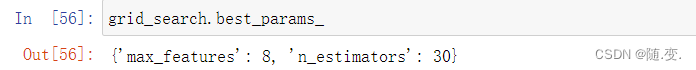
grid_search = GridSearchCV(forest_reg, param_grid, cv=5,
scoring='neg_mean_squared_error',
return_train_score=True)
grid_search.fit(housing_prepared, housing_labels)然后可以获得最佳参数:
分析最佳模型和误差
feature_importances = grid_search.best_estimator_.feature_importances_
extra_attribs = ["rooms_per_hhold", "pop_per_hhold", "bedrooms_per_room"]
#cat_encoder = cat_pipeline.named_steps["cat_encoder"] # old solution
cat_encoder = full_pipeline.named_transformers_["cat"]
cat_one_hot_attribs = list(cat_encoder.categories_[0])
attributes = num_attribs + extra_attribs + cat_one_hot_attribs
sorted(zip(feature_importances, attributes), reverse=True)
通过测试集评估系统
final_model = grid_search.best_estimator_

X_test = strat_test_set.drop("median_house_value", axis=1)
y_test = strat_test_set["median_house_value"].copy()

X_test_prepared = full_pipeline.transform(X_test)
final_predictions = final_model.predict(X_test_prepared)

final_mse = mean_squared_error(y_test, final_predictions)
final_rmse = np.sqrt(final_mse)
final_rmse![]()
如此一个初步的系统就完成了。后面是将系统上线 ,监控并维护。


 3741
3741


 被折叠的 条评论
为什么被折叠?
被折叠的 条评论
为什么被折叠?
 到【灌水乐园】发言


