


目录
1.2.4.全连接层(Fully Connected Layer)
一.卷积神经网络(CNN)-图片分类和验证码识别
1.1.使用Python处理图片
在具体介绍 CNN 之前,我们先来看看怎样使用 Python 处理图片。Python 处理图片最主要使用的类库是 Pillow (Python2 PIL 的 fork),使用以下命令即可安装:
pip3 install Pillow
一些简单操作的例子如下,如果你想了解更多可以参考 Pillow 的文档:
# 打开图片
>>> from PIL import Image
>>> img = Image.open("1.png")

# 查看图片信息
>>> img.size
(175, 230)
>>> img.mode
'RGB'
>>> img
<PIL.PngImagePlugin.PngImageFile image mode=RGB size=175x230 at 0x10B807B50>

# 缩放图片
>>> img1 = img.resize((20, 30))
>>> img1
<PIL.Image.Image image mode=RGB size=20x30 at 0x106426FD0>

# 裁剪图片
>>> img2 = img.crop((0, 0, 16, 16))
>>> img2
<PIL.Image.Image image mode=RGB size=16x16 at 0x105E0EFD0>

# 保存图片
>>> img1.save("11.png")
>>> img2.save("12.png")
使用 pytorch 处理图片时要首先获取图片的数据,即各个像素对应的颜色值,例如大小为 175 * 230,模式是 RGB 的图片会拥有 175 * 230 * 3 的数据,3 分别代表红绿蓝的值,范围是 0 ~ 255,把图片转换为 pytorch 的 tensor 对象需要经过 numpy 中转,以下是转换的例子:
>>> import numpy
>>> import torch
>>> v = numpy.asarray(img)
>>> t = torch.tensor(v)
>>> t
tensor([[[255, 253, 254],
         [255, 253, 254],
         [255, 253, 254],
         ...,
         [255, 253, 254],
         [255, 253, 254],
         [255, 253, 254]],

        [[255, 253, 254],
         [255, 253, 254],
         [255, 253, 254],
         ...,
         [255, 253, 254],
         [255, 253, 254],
         [255, 253, 254]],

        [[255, 253, 254],
         [255, 253, 254],
         [255, 253, 254],
         ...,
         [255, 253, 254],
         [255, 253, 254],
         [255, 253, 254]],

        ...,

        [[255, 253, 254],
         [255, 253, 254],
         [255, 253, 254],
         ...,
         [255, 253, 254],
         [255, 253, 254],
         [255, 253, 254]],

        [[255, 253, 254],
         [255, 253, 254],
         [255, 253, 254],
         ...,
         [255, 253, 254],
         [255, 253, 254],
         [255, 253, 254]],

        [[255, 253, 254],
         [255, 253, 254],
         [255, 253, 254],
         ...,
         [255, 253, 254],
         [255, 253, 254],
         [255, 253, 254]]], dtype=torch.uint8)
>>> t.shape
torch.Size([230, 175, 3])
可以看到 tensor 的维度是 高度 x 宽度 x 通道数 (RGB 图片为 3,黑白图片为 1),可是 pytorch 的 CNN 模型会要求维度为 通道数 x 宽度 x 高度,并且数值应该正规化到 0 ~ 1 的范围内,使用以下代码可以实现:
# 交换维度 0 (高度) 和 维度 2 (通道数)
>>> t1 = t.transpose(0, 2)
>>> t1.shape
torch.Size([3, 175, 230])

>>> t2 = t1 / 255.0
>>> t2
tensor([[[1.0000, 1.0000, 1.0000,  ..., 1.0000, 1.0000, 1.0000],
         [1.0000, 1.0000, 1.0000,  ..., 1.0000, 1.0000, 1.0000],
         [1.0000, 1.0000, 1.0000,  ..., 1.0000, 1.0000, 1.0000],
         ...,
         [1.0000, 1.0000, 1.0000,  ..., 1.0000, 1.0000, 1.0000],
         [1.0000, 1.0000, 1.0000,  ..., 1.0000, 1.0000, 1.0000],
         [1.0000, 1.0000, 1.0000,  ..., 1.0000, 1.0000, 1.0000]],

        [[0.9922, 0.9922, 0.9922,  ..., 0.9922, 0.9922, 0.9922],
         [0.9922, 0.9922, 0.9922,  ..., 0.9922, 0.9922, 0.9922],
         [0.9922, 0.9922, 0.9922,  ..., 0.9922, 0.9922, 0.9922],
         ...,
         [0.9922, 0.9922, 0.9922,  ..., 0.9922, 0.9922, 0.9922],
         [0.9922, 0.9922, 0.9922,  ..., 0.9922, 0.9922, 0.9922],
         [0.9922, 0.9922, 0.9922,  ..., 0.9922, 0.9922, 0.9922]],

        [[0.9961, 0.9961, 0.9961,  ..., 0.9961, 0.9961, 0.9961],
         [0.9961, 0.9961, 0.9961,  ..., 0.9961, 0.9961, 0.9961],
         [0.9961, 0.9961, 0.9961,  ..., 0.9961, 0.9961, 0.9961],
         ...,
         [0.9961, 0.9961, 0.9961,  ..., 0.9961, 0.9961, 0.9961],
         [0.9961, 0.9961, 0.9961,  ..., 0.9961, 0.9961, 0.9961],
         [0.9961, 0.9961, 0.9961,  ..., 0.9961, 0.9961, 0.9961]]])
之后就可以围绕类似上面例子中 t2 这样的 tensor 对象做文章了🥳。
1.2.卷积神经网络(CNN)
1.2.1简介
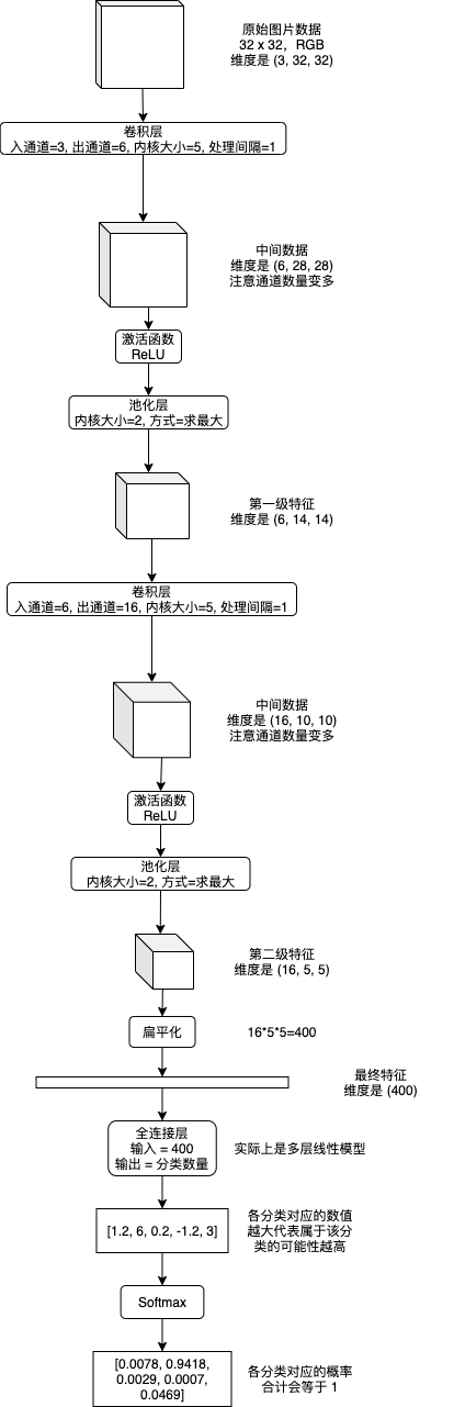
卷积神经网络 (CNN) 会从图片的各个部分提取特征,然后再从一级特征提取二级特征,如有必要再提取三级特征 (以此类推),提取结束以后扁平化到最终特征,然后使用多层或单层线性模型来实现分类识别。提取各级特征会使用卷积层 (Convolution Layer) 和池化层 (Pooling Layer),提取特征时可以选择添加通道数量以增加各个部分的信息量,分类识别最终特征使用的线性模型又称全连接层 (Fully Connected Layer),下图是流程示例:
之前的文章介绍线性模型和递归模型的时候我使用了数学公式,但只用数学公式说明 CNN 将会非常难以理解,所以接下来我会伴随例子逐步讲解各个层具体做了怎样的运算。
1.2.2.卷积层(Convolution layer)
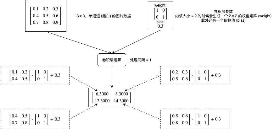
卷积层会对图片的各个部分做矩阵乘法操作,然后把结果作为一个新的矩阵,每个卷积层有两个主要的参数,一个是内核大小 (kernel_size),一个是处理间隔 (stride),下图是一个非常简单的计算流程例子:
如果增加处理间隔会怎样呢?下图展示了不同处理间隔的计算部分和输出结果维度的区别:
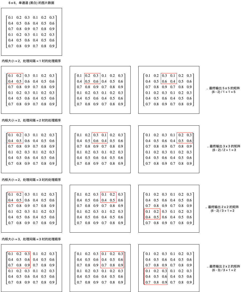
我们可以看到处理间隔决定了每次向右或者向下移动的距离,输出长度可以使用公式 (长度 - 内核大小) / 处理间隔 + 1 计算,输出宽度可以使用公式 (长度 - 内核大小) / 处理间隔 + 1 计算。
现在再来看看 pytorch 中怎样使用卷积层,创建卷积层可以使用 torch.nn.Conv2d:
# 创建卷积层,入通道 = 1,出通道 = 1,内核大小 = 2,处理间隔 = 1
>>> conv2d = torch.nn.Conv2d(in_channels = 1, out_channels = 1, kernel_size = 2, stride = 1)

# 查看卷积层内部的参数,第一个是内核对应的权重矩阵,第二个是偏移值
>>> p = list(conv2d.parameters())
>>> p
[Parameter containing:
tensor([[[[-0.0650, -0.0575],
          [-0.0313, -0.3539]]]], requires_grad=True), Parameter containing:
tensor([0.1482], requires_grad=True)]

# 现在生成一个 5 x 5,单通道的图片数据,为了方便理解这里使用了 1 ~ 25,实际应该使用 0 ~ 1 之间的值
>>> x = torch.tensor(list(range(1, 26)), dtype=torch.float).reshape(1, 1, 5, 5)
>>> x
tensor([[[[ 1.,  2.,  3.,  4.,  5.],
          [ 6.,  7.,  8.,  9., 10.],
          [11., 12., 13., 14., 15.],
          [16., 17., 18., 19., 20.],
          [21., 22., 23., 24., 25.]]]])

# 使用卷积层计算输出
>>> y = conv2d(x)
>>> y
tensor([[[[ -2.6966,  -3.2043,  -3.7119,  -4.2196],
          [ -5.2349,  -5.7426,  -6.2502,  -6.7579],
          [ -7.7732,  -8.2809,  -8.7885,  -9.2962],
          [-10.3115, -10.8192, -11.3268, -11.8345]]]],
       grad_fn=<MkldnnConvolutionBackward>)

# 我们可以模拟一下处理单个部分的计算,看看和上面的输出是否一致

# 第 1 部分
>>> x[0,0,0:2,0:2]
tensor([[1., 2.],
        [6., 7.]])
>>> (p[0][0,0,:,:] * x[0,0,0:2,0:2]).sum() + p[1]
tensor([-2.6966], grad_fn=<AddBackward0>)

# 第 2 部分
>>> x[0,0,0:2,1:3]
tensor([[2., 3.],
        [7., 8.]])
>>> (p[0][0,0,:,:] * x[0,0,0:2,1:3]).sum() + p[1]
tensor([-3.2043], grad_fn=<AddBackward0>)

# 第 3 部分
>>> (p[0][0,0,:,:] * x[0,0,0:2,2:4]).sum() + p[1]
tensor([-3.7119], grad_fn=<AddBackward0>)

# 一致吧🥳
到这里你应该了解单通道的卷积层是怎样计算的,那么多通道呢?如果有多个入通道,那么卷积层的权重矩阵会相应有多份,如果有多个出通道,那么卷积层的权重矩阵数量也会乘以出通道的倍数,例如有 3 个入通道,2 个出通道时,卷积层的权重矩阵会有 6 个 (3 * 2),偏移值会有 2 个,计算规则如下:
部分输出[出通道1] = 部分输入[入通道1] * 权重矩阵[0][0] + 部分输入[入通道2] * 权重矩阵[0][1] + 部分输入[入通道3] * 权重矩阵[0][2] + 偏移值1
部分输出[出通道2] = 部分输入[入通道1] * 权重矩阵[1][0] + 部分输入[入通道2] * 权重矩阵[1][1] + 部分输入[入通道3] * 权重矩阵[1][2] + 偏移值2
从计算规则可以看出,出通道越多每个部分可提取的特征数量 (信息量) 也就越多,但计算量也会相应增大。
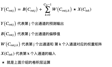
最后看看卷积层的数学公式 (基本和 pytorch 文档的公式相同),现在应该可以理解了吧🤢?
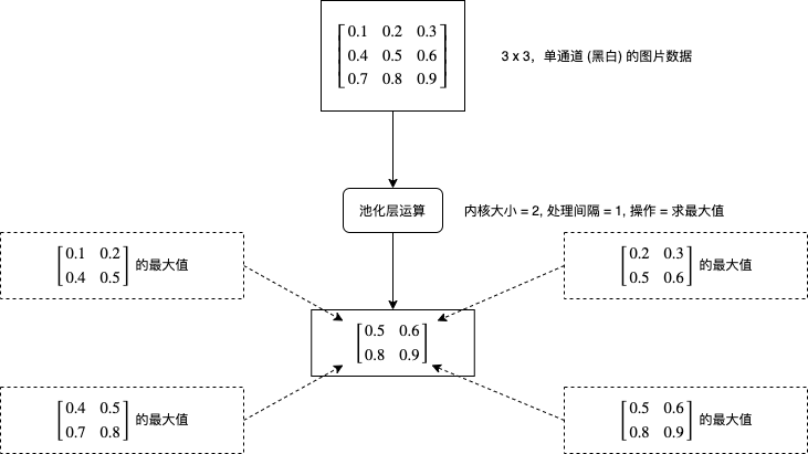
1.2.3.池化层(Pooling layer)
池化层的处理比较好理解,它会对每个图片每个区域进行求最大值或者求平均值等运算,如下图所示:
现在再来看看 pytorch 中怎样使用卷积层,创建求最大值的池化层可以使用 torch.nn.MaxPool2d,创建求平均值的池化层可以使用 torch.nn.AvgPool2d:
# 创建池化层,内核大小 = 2,处理间隔 = 2
>>> maxPool = torch.nn.MaxPool2d(2, stride=2)

# 生成一个 6 x 6,单通道的图片数据
>>> x = torch.tensor(range(1, 37), dtype=float).reshape(1, 1, 6, 6)
>>> x
tensor([[[[ 1.,  2.,  3.,  4.,  5.,  6.],
          [ 7.,  8.,  9., 10., 11., 12.],
          [13., 14., 15., 16., 17., 18.],
          [19., 20., 21., 22., 23., 24.],
          [25., 26., 27., 28., 29., 30.],
          [31., 32., 33., 34., 35., 36.]]]], dtype=torch.float64)

# 使用池化层计算输出
>>> maxPool(x)
tensor([[[[ 8., 10., 12.],
          [20., 22., 24.],
          [32., 34., 36.]]]], dtype=torch.float64)

# 很好理解吧🥳

# 创建和使用求平均值的池化层也很简单
>>> avgPool = torch.nn.AvgPool2d(2, stride=2)
>>> avgPool(x)
tensor([[[[ 4.5000,  6.5000,  8.5000],
          [16.5000, 18.5000, 20.5000],
          [28.5000, 30.5000, 32.5000]]]], dtype=torch.float64)
1.2.4.全连接层(Fully Connected Layer)
全连接层实际上就是多层或单层线性模型,但把特征传到全连接层之前还需要进行扁平化 (Flatten),例子如下所示:
# 模拟创建一个批次数量为 2,通道数为 3,长宽各为 2 的特征
>>> x = torch.rand((2, 3, 2, 2))
>>> x
tensor([[[[0.6395, 0.6240],
          [0.4194, 0.6054]],

         [[0.4798, 0.4690],
          [0.2647, 0.6087]],

         [[0.5727, 0.7567],
          [0.8287, 0.1382]]],


        [[[0.7903, 0.8635],
          [0.0053, 0.6417]],

         [[0.7093, 0.7740],
          [0.3115, 0.7587]],

         [[0.5875, 0.8268],
          [0.2923, 0.6016]]]])

# 对它进行扁平化,维度会变为 批次数量, 通道数*长*宽
>>> x_flatten = x.view(x.shape[0], -1)
>>> x_flatten
tensor([[0.6395, 0.6240, 0.4194, 0.6054, 0.4798, 0.4690, 0.2647, 0.6087, 0.5727,
         0.7567, 0.8287, 0.1382],
        [0.7903, 0.8635, 0.0053, 0.6417, 0.7093, 0.7740, 0.3115, 0.7587, 0.5875,
         0.8268, 0.2923, 0.6016]])

# 之后再传给线性模型即可
>>> linear = torch.nn.Linear(in_features=12, out_features=2)
>>> linear(x_flatten)
tensor([[-0.3067, -0.5534],
        [-0.1876, -0.6523]], grad_fn=<AddmmBackward>)
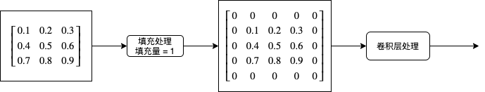
1.2.5.填充处理
在看前面提到的卷积层操作的时候,你可能会发现如果处理间隔 (stride) 小于内核大小 (kernel_size),那么图片边缘的像素参与运算的次数会比图片中间的像素要少,也就是说图片边缘对运算结果的影响会更小,如果图片边缘的信息同样比较重要,那么就会影响预测输出的精度。为了解决这个问题发明的就是填充处理,填充处理简单的来说就是在卷积层初期前给图片的周边添加 0,如果填充量等于 1,那么长宽会各增加 2,如下图所示:
在 pytorch 中添加填充处理可以在创建 Conv2d 的时候指定 padding 参数:
# 创建卷积层,入通道 = 1,出通道 = 1,内核大小 = 2,处理间隔 = 1, 填充量 = 1
>>> conv2d = torch.nn.Conv2d(in_channels = 1, out_channels = 1, kernel_size = 2, stride = 1, padding = 1)
1.3.使用CNN实现图片分类(LeNet)
接下来我们试试使用 CNN 实现图片分类,也就是给出一张图片让程序识别里面的是什么东西,使用的数据集是 cifar-10,这是一个很经典的数据集,包含了 60000 张 32x32 的小图片,图片有十个分类 (飞机,汽车,鸟,猫,鹿,狗,青蛙,马,船,货车),官方下载地址在这里。

需要注意的是,官方下载地址只包含二进制数据,通常很多文章或者教程都会让我们使用 torchvision.datasets.CIFAR10 等现成的加载器来加载这个数据集,但我不推荐使用这种方法,因为如果我们需要训练实际业务上的数据,那么肯定不会有现成的加载器可以用,还是得一张张图片的加载和转换。所以这里我使用了 cifar-10 的原始图片库,然后演示怎样从代码加载图片和标签,然后转换到训练使用的 tensor 对象。
以下的代码使用了 LeNet 模型,这是 30 年前就已经被提出的模型,结构和本文第一个图片介绍的一样。此外还有一些需要注意的地方:
- cifar-10 官方默认划分了 50000 张图片作为训练集,10000 张图片作为验证集;而我的代码划分了 48000 张图片作为训练集,6000 张图片作为验证集,6000 张图片作为测试集,所以正确率等数据会和其他文章或者论文不一致
- 训练时的损失计算器使用了
CrossEntropyLoss, 这个计算器的特征是要求预测输出是 onehot,实际输出是索引值 (只有一个分类是正确输出),例如图片分类为鸟时,预测输出应该为[0, 0, 1, 0, 0, 0, 0, 0, 0, 0]实际输出应该为2 - 转换各个分类的数值到概率使用了 Softmax 函数, 这个函数必须放在模型之外,如果放在模型内部会导致训练效果变差,因为
CrossEntropyLoss损失计算器会尽量让正确输出的数值更高,错误输出的数值更低,而不是分别接近 1 和 0,使用 softmax 会干扰损失的计算
import os
import sys
import torch
import gzip
import itertools
import random
import numpy
import json
from PIL import Image
from torch import nn
from matplotlib import pyplot

# 分析目标的图片大小,全部图片都会先缩放到这个大小
IMAGE_SIZE = (32, 32)
# 分析目标的图片所在的文件夹
IMAGE_DIR = "./cifar"
# 包含所有图片标签的文本文件
IMAGE_LABELS_PATH = "./cifar/labels.txt"

class MyModel(nn.Module):
    """图片分类 (LeNet)"""
    def __init__(self, num_labels):
        super().__init__()
        # 卷积层和池化层
        self.cnn_model = nn.Sequential(
            nn.Conv2d(3, 6, kernel_size=5), # 维度: B,3,32,32 => B,6,28,28
            nn.ReLU(),
            nn.MaxPool2d(2, stride=2), # 维度: B,6,14,14
            nn.Conv2d(6, 16, kernel_size=5), # 维度: B,16,10,10
            nn.ReLU(),
            nn.MaxPool2d(2, stride=2) # 维度: B,16,5,5
        )
        # 全连接层
        self.fc_model = nn.Sequential(
            nn.Linear(16 * 5 * 5, 120), # 维度: B,120
            nn.ReLU(),
            nn.Dropout(0.1),
            nn.Linear(120, 60), # 维度: B,60
            nn.ReLU(),
            nn.Dropout(0.1),
            nn.Linear(60, num_labels), # 维度: B,num_labels
        )

    def forward(self, x):
        # 应用卷积层和池化层
        cnn_features = self.cnn_model(x)
        # 扁平化输出的特征
        cnn_features_flatten = cnn_features.view(cnn_features.shape[0], -1)
        # 应用全连接层
        y = self.fc_model(cnn_features_flatten)
        return y

def save_tensor(tensor, path):
    """保存 tensor 对象到文件"""
    torch.save(tensor, gzip.GzipFile(path, "wb"))

def load_tensor(path):
    """从文件读取 tensor 对象"""
    return torch.load(gzip.GzipFile(path, "rb"))

def image_to_tensor(img):
    """转换图片对象到 tensor 对象"""
    in_img = img.resize(IMAGE_SIZE)
    arr = numpy.asarray(in_img)
    t = torch.from_numpy(arr)
    t = t.transpose(0, 2) # 转换维度 H,W,C 到 C,W,H
    t = t / 255.0 # 正规化数值使得范围在 0 ~ 1
    return t

def load_image_labels():
    """读取图片分类列表"""
    return list(filter(None, open(IMAGE_LABELS_PATH).read().split()))

def prepare_save_batch(batch, tensor_in, tensor_out):
    """准备训练 - 保存单个批次的数据"""
    # 切分训练集 (80%),验证集 (10%) 和测试集 (10%)
    random_indices = torch.randperm(tensor_in.shape[0])
    training_indices = random_indices[:int(len(random_indices)*0.8)]
    validating_indices = random_indices[int(len(random_indices)*0.8):int(len(random_indices)*0.9):]
    testing_indices = random_indices[int(len(random_indices)*0.9):]
    training_set = (tensor_in[training_indices], tensor_out[training_indices])
    validating_set = (tensor_in[validating_indices], tensor_out[validating_indices])
    testing_set = (tensor_in[testing_indices], tensor_out[testing_indices])

    # 保存到硬盘
    save_tensor(training_set, f"data/training_set.{batch}.pt")
    save_tensor(validating_set, f"data/validating_set.{batch}.pt")
    save_tensor(testing_set, f"data/testing_set.{batch}.pt")
    print(f"batch {batch} saved")

def prepare():
    """准备训练"""
    # 数据集转换到 tensor 以后会保存在 data 文件夹下
    if not os.path.isdir("data"):
        os.makedirs("data")

    # 准备图片分类到序号的索引
    labels_to_index = { label: index for index, label in enumerate(load_image_labels()) }

    # 查找所有图片
    image_paths = []
    for root, dirs, files in os.walk(IMAGE_DIR):
        for filename in files:
            path = os.path.join(root, filename)
            if not path.endswith(".png"):
                continue
            # 分类名称在文件名中,例如
            # 2598_cat.png => cat
            label = filename.split(".")[0].split("_")[1]
            label_index = labels_to_index.get(label)
            if label_index is None:
                continue
            image_paths.append((path, label_index))

    # 打乱图片顺序
    random.shuffle(image_paths)

    # 分批读取和保存图片
    batch_size = 1000
    for batch in range(0, len(image_paths) // batch_size):
        image_tensors = []
        image_labels = []
        for path, label_index in image_paths[batch*batch_size:(batch+1)*batch_size]:
            with Image.open(path) as img:
                t = image_to_tensor(img)
                image_tensors.append(t)
            image_labels.append(label_index)
        tensor_in = torch.stack(image_tensors) # 维度: B,C,W,H
        tensor_out = torch.tensor(image_labels) # 维度: B
        prepare_save_batch(batch, tensor_in, tensor_out)

def train():
    """开始训练"""
    # 创建模型实例
    num_labels = len(load_image_labels())
    model = MyModel(num_labels)

    # 创建损失计算器
    # 计算单分类输出最好使用 CrossEntropyLoss, 多分类输出最好使用 BCELoss
    # 使用 CrossEntropyLoss 时实际输出应该为标签索引值,不需要转换为 onehot
    loss_function = torch.nn.CrossEntropyLoss()

    # 创建参数调整器
    optimizer = torch.optim.Adam(model.parameters())

    # 记录训练集和验证集的正确率变化
    training_accuracy_history = []
    validating_accuracy_history = []

    # 记录最高的验证集正确率
    validating_accuracy_highest = -1
    validating_accuracy_highest_epoch = 0

    # 读取批次的工具函数
    def read_batches(base_path):
        for batch in itertools.count():
            path = f"{base_path}.{batch}.pt"
            if not os.path.isfile(path):
                break
            yield load_tensor(path)

    # 计算正确率的工具函数
    def calc_accuracy(actual, predicted):
        # 把最大的值当作正确分类,然后比对有多少个分类相等
        predicted_labels = predicted.argmax(dim=1)
        acc = (actual == predicted_labels).sum().item() / actual.shape[0]
        return acc

    # 划分输入和输出的工具函数
    def split_batch_xy(batch, begin=None, end=None):
        # shape = batch_size, channels, width, height
        batch_x = batch[0][begin:end]
        # shape = batch_size
        batch_y = batch[1][begin:end]
        return batch_x, batch_y

    # 开始训练过程
    for epoch in range(1, 10000):
        print(f"epoch: {epoch}")

        # 根据训练集训练并修改参数
        # 切换模型到训练模式,将会启用自动微分,批次正规化 (BatchNorm) 与 Dropout
        model.train()
        training_accuracy_list = []
        for batch_index, batch in enumerate(read_batches("data/training_set")):
            # 切分小批次,有助于泛化模型
            training_batch_accuracy_list = []
            for index in range(0, batch[0].shape[0], 100):
                # 划分输入和输出
                batch_x, batch_y = split_batch_xy(batch, index, index+100)
                # 计算预测值
                predicted = model(batch_x)
                # 计算损失
                loss = loss_function(predicted, batch_y)
                # 从损失自动微分求导函数值
                loss.backward()
                # 使用参数调整器调整参数
                optimizer.step()
                # 清空导函数值
                optimizer.zero_grad()
                # 记录这一个批次的正确率,torch.no_grad 代表临时禁用自动微分功能
                with torch.no_grad():
                    training_batch_accuracy_list.append(calc_accuracy(batch_y, predicted))
            # 输出批次正确率
            training_batch_accuracy = sum(training_batch_accuracy_list) / len(training_batch_accuracy_list)
            training_accuracy_list.append(training_batch_accuracy)
            print(f"epoch: {epoch}, batch: {batch_index}: batch accuracy: {training_batch_accuracy}")
        training_accuracy = sum(training_accuracy_list) / len(training_accuracy_list)
        training_accuracy_history.append(training_accuracy)
        print(f"training accuracy: {training_accuracy}")

        # 检查验证集
        # 切换模型到验证模式,将会禁用自动微分,批次正规化 (BatchNorm) 与 Dropout
        model.eval()
        validating_accuracy_list = []
        for batch in read_batches("data/validating_set"):
            batch_x, batch_y = split_batch_xy(batch)
            predicted = model(batch_x)
            validating_accuracy_list.append(calc_accuracy(batch_y, predicted))
        validating_accuracy = sum(validating_accuracy_list) / len(validating_accuracy_list)
        validating_accuracy_history.append(validating_accuracy)
        print(f"validating accuracy: {validating_accuracy}")

        # 记录最高的验证集正确率与当时的模型状态,判断是否在 20 次训练后仍然没有刷新记录
        if validating_accuracy > validating_accuracy_highest:
            validating_accuracy_highest = validating_accuracy
            validating_accuracy_highest_epoch = epoch
            save_tensor(model.state_dict(), "model.pt")
            print("highest validating accuracy updated")
        elif epoch - validating_accuracy_highest_epoch > 20:
            # 在 20 次训练后仍然没有刷新记录,结束训练
            print("stop training because highest validating accuracy not updated in 20 epoches")
            break

    # 使用达到最高正确率时的模型状态
    print(f"highest validating accuracy: {validating_accuracy_highest}",
        f"from epoch {validating_accuracy_highest_epoch}")
    model.load_state_dict(load_tensor("model.pt"))

    # 检查测试集
    testing_accuracy_list = []
    for batch in read_batches("data/testing_set"):
        batch_x, batch_y = split_batch_xy(batch)
        predicted = model(batch_x)
        testing_accuracy_list.append(calc_accuracy(batch_y, predicted))
    testing_accuracy = sum(testing_accuracy_list) / len(testing_accuracy_list)
    print(f"testing accuracy: {testing_accuracy}")

    # 显示训练集和验证集的正确率变化
    pyplot.plot(training_accuracy_history, label="training")
    pyplot.plot(validating_accuracy_history, label="validing")
    pyplot.ylim(0, 1)
    pyplot.legend()
    pyplot.show()

def eval_model():
    """使用训练好的模型"""
    # 创建模型实例,加载训练好的状态,然后切换到验证模式
    labels = load_image_labels()
    num_labels = len(labels)
    model = MyModel(num_labels)
    model.load_state_dict(load_tensor("model.pt"))
    model.eval()

    # 询问图片路径,并显示可能的分类一览
    while True:
        try:
            # 构建输入
            image_path = input("Image path: ")
            if not image_path:
                continue
            with Image.open(image_path) as img:
                tensor_in = image_to_tensor(img).unsqueeze(0) # 维度 C,W,H => 1,C,W,H
            # 预测输出
            tensor_out = model(tensor_in)
            # 转换到各个分类对应的概率
            tensor_out = nn.functional.softmax(tensor_out, dim=1)
            # 显示按概率排序后的分类一览
            rates = (t.item() for t in tensor_out[0])
            label_with_rates = list(zip(labels, rates))
            label_with_rates.sort(key=lambda p:-p[1])
            for label, rate in label_with_rates[:5]:
                rate = rate * 100
                print(f"{label}: {rate:0.2f}%")
            print()
        except Exception as e:
            print("error:", e)

def main():
    """主函数"""
    if len(sys.argv) < 2:
        print(f"Please run: {sys.argv[0]} prepare|train|eval")
        exit()

    # 给随机数生成器分配一个初始值,使得每次运行都可以生成相同的随机数
    # 这是为了让过程可重现,你也可以选择不这样做
    random.seed(0)
    torch.random.manual_seed(0)

    # 根据命令行参数选择操作
    operation = sys.argv[1]
    if operation == "prepare":
        prepare()
    elif operation == "train":
        train()
    elif operation == "eval":
        eval_model()
    else:
        raise ValueError(f"Unsupported operation: {operation}")

if __name__ == "__main__":
    main()
准备训练使用的数据和开始训练需要分别执行以下命令:
python3 example.py prepare
python3 example.py train
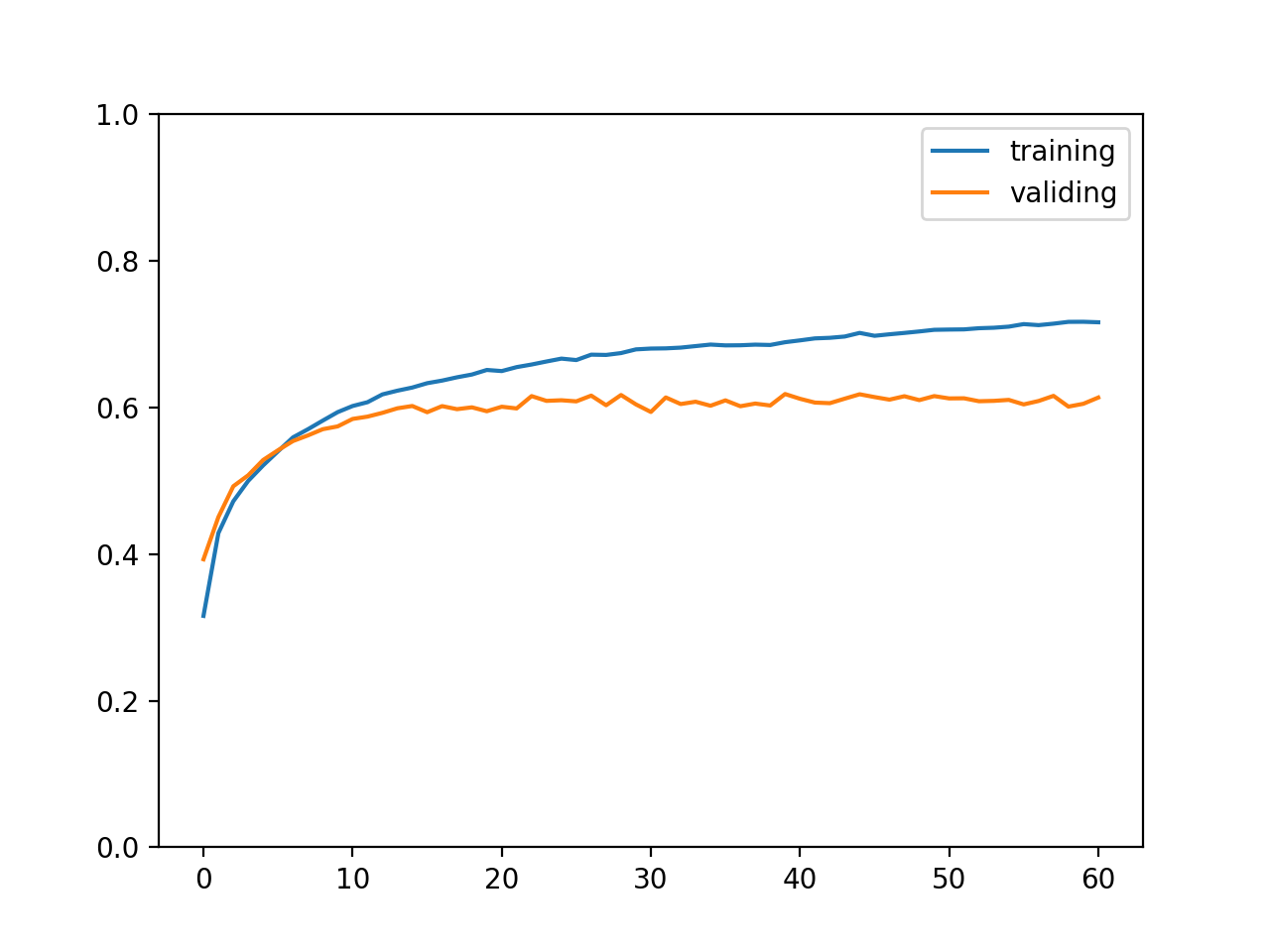
最终输出结果如下,可以看到训练集正确率达到了 71%,验证集和测试集正确率达到了 61%,这个正确率代表可以精准说出图片所属的分类,也称 top 1 正确率;此外计算正确分类在概率排前三的分类之中的比率称为 top 3 正确率,如果是电商上传图片以后给出三个可能的商品分类让商家选择,那么计算 top 3 正确率就有意义了。
training accuracy: 0.7162083333333331
validating accuracy: 0.6134999999999998
stop training because highest validating accuracy not updated in 20 epoches
highest validating accuracy: 0.6183333333333333 from epoch 40
testing accuracy: 0.6168333333333332
训练集与验证集正确率变化如下图所示:
实际使用模型的例子如下,输出代表预测图片有 79.23% 的概率是飞机,你也可以试试在互联网上随便找一张图片让这个模型识别:
$ python3 example.py eval
Image path: ./cifar/test/2257_airplane.png
airplane: 79.23%
deer: 6.06%
automobile: 4.04%
cat: 2.89%
frog: 2.11%
1.4.使用CNN实现图片分类(ResNet)
上述的模型 top 1 正确率只达到了 61%, 毕竟是 30 年前的老模型了🧔,这里我再介绍一个相对比较新的模型,ResNet 是在 2015 年中提出的模型,论文地址在这里,特征是会把输入和输出结合在一块,例如原来计算 y = f(x) 会变为 y = f(x) + x,从而抵消层数变多带来的梯度消失问题 (参考我之前写的训练过程中常用的技巧)。
下图是 ResNet-18 模型的结构,内部可以分为 4 组,每个组都包括 2 个基础块和 4 个卷积层,并且每个基础块会把输入和输出结合在一起,层数合计一共有 16,加上最开始转换输入的层和全连接层一共有 18 层,所以称为 ResNet-18,除此之外还有 ResNet-34,ResNet-50 等等变种,如果有兴趣可以参考本节末尾给出的 torchvision 的实现代码。
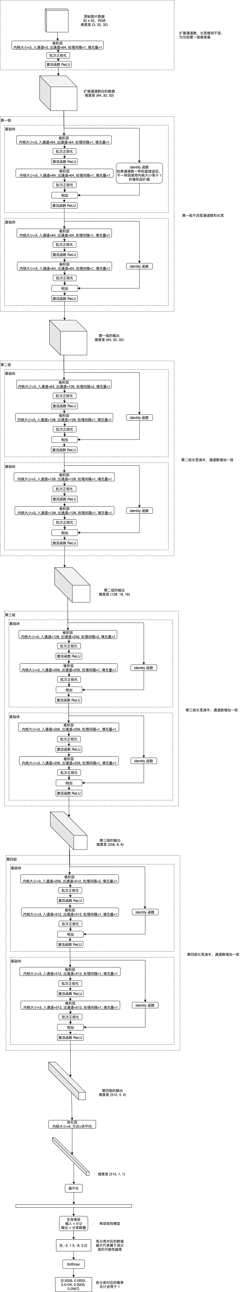
从图中可以看到,从第二组开始会把长宽变为一半,同时通道数增加一倍,然后维持通道数和长宽不变,所有组结束后使用一个 AvgPool2d 来让长宽强制变为 1x1,最后交给全连接层。计算卷积层输出长宽的公式是 (长度 - 内核大小 + 填充量*2) / 处理间隔 + 1,让长宽变为一半会使用内核大小 3,填充量 1,处理间隔 2 ,例如长度为 32 可以计算得出 (32 - 3 + 2) / 2 + 1 == 16;而维持长宽的则会使用内核大小 3,填充量 1,处理间隔 1,例如长度为 32 可以计算得出 (32 - 3 + 2) / 1 + 1 == 32。
以下是使用 ResNet-18 进行训练的代码:
import os
import sys
import torch
import gzip
import itertools
import random
import numpy
import json
from PIL import Image
from torch import nn
from matplotlib import pyplot

# 分析目标的图片大小,全部图片都会先缩放到这个大小
IMAGE_SIZE = (32, 32)
# 分析目标的图片所在的文件夹
IMAGE_DIR = "./cifar"
# 包含所有图片标签的文本文件
IMAGE_LABELS_PATH = "./cifar/labels.txt"

class BasicBlock(nn.Module):
    """ResNet 使用的基础块"""
    expansion = 1 # 定义这个块的实际出通道是 channels_out 的几倍,这里的实现固定是一倍
    def __init__(self, channels_in, channels_out, stride):
        super().__init__()
        # 生成 3x3 的卷积层
        # 处理间隔 stride = 1 时,输出的长宽会等于输入的长宽,例如 (32-3+2)//1+1 == 32
        # 处理间隔 stride = 2 时,输出的长宽会等于输入的长宽的一半,例如 (32-3+2)//2+1 == 16
        # 此外 resnet 的 3x3 卷积层不使用偏移值 bias
        self.conv1 = nn.Sequential(
            nn.Conv2d(channels_in, channels_out, kernel_size=3, stride=stride, padding=1, bias=False),
            nn.BatchNorm2d(channels_out))
        # 再定义一个让输出和输入维度相同的 3x3 卷积层
        self.conv2 = nn.Sequential(
            nn.Conv2d(channels_out, channels_out, kernel_size=3, stride=1, padding=1, bias=False),
            nn.BatchNorm2d(channels_out))
        # 让原始输入和输出相加的时候,需要维度一致,如果维度不一致则需要整合
        self.identity = nn.Sequential()
        if stride != 1 or channels_in != channels_out * self.expansion:
            self.identity = nn.Sequential(
                nn.Conv2d(channels_in, channels_out * self.expansion, kernel_size=1, stride=stride, bias=False),
                nn.BatchNorm2d(channels_out * self.expansion))

    def forward(self, x):
        # x => conv1 => relu => conv2 => + => relu
        # |                              ^
        # |==============================|
        tmp = self.conv1(x)
        tmp = nn.functional.relu(tmp)
        tmp = self.conv2(tmp)
        tmp += self.identity(x)
        y = nn.functional.relu(tmp)
        return y

class MyModel(nn.Module):
    """图片分类 (ResNet-18)"""
    def __init__(self, num_labels, block_type = BasicBlock):
        super().__init__()
        # 记录上一层的出通道数量
        self.previous_channels_out = 64
        # 把 3 通道转换到 64 通道,长宽不变
        self.conv1 = nn.Sequential(
            nn.Conv2d(3, self.previous_channels_out, kernel_size=3, stride=1, padding=1, bias=False),
            nn.BatchNorm2d(self.previous_channels_out))
        # ResNet 使用的各个层
        self.layer1 = self._make_layer(block_type, channels_out=64, num_blocks=2, stride=1)
        self.layer2 = self._make_layer(block_type, channels_out=128, num_blocks=2, stride=2)
        self.layer3 = self._make_layer(block_type, channels_out=256, num_blocks=2, stride=2)
        self.layer4 = self._make_layer(block_type, channels_out=512, num_blocks=2, stride=2)
        # 把最后一层的长宽转换为 1x1 的池化层,Adaptive 表示会自动检测原有长宽
        # 例如 B,512,4,4 的矩阵会转换为 B,512,1,1,每个通道的单个值会是原有 16 个值的平均
        self.avgPool = nn.AdaptiveAvgPool2d((1, 1))
        # 全连接层,只使用单层线性模型
        self.fc_model = nn.Linear(512 * block_type.expansion, num_labels)

    def _make_layer(self, block_type, channels_out, num_blocks, stride):
        blocks = []
        # 添加第一个块
        blocks.append(block_type(self.previous_channels_out, channels_out, stride))
        self.previous_channels_out = channels_out * block_type.expansion
        # 添加剩余的块,剩余的块固定处理间隔为 1,不会改变长宽
        for _ in range(num_blocks-1):
            blocks.append(block_type(self.previous_channels_out, self.previous_channels_out, 1))
            self.previous_channels_out *= block_type.expansion
        return nn.Sequential(*blocks)

    def forward(self, x):
        # 转换出通道到 64
        tmp = self.conv1(x)
        tmp = nn.functional.relu(tmp)
        # 应用 ResNet 的各个层
        tmp = self.layer1(tmp)
        tmp = self.layer2(tmp)
        tmp = self.layer3(tmp)
        tmp = self.layer4(tmp)
        # 转换长宽到 1x1
        tmp = self.avgPool(tmp)
        # 扁平化,维度会变为 B,512
        tmp = tmp.view(tmp.shape[0], -1)
        # 应用全连接层
        y = self.fc_model(tmp)
        return y

def save_tensor(tensor, path):
    """保存 tensor 对象到文件"""
    torch.save(tensor, gzip.GzipFile(path, "wb"))

def load_tensor(path):
    """从文件读取 tensor 对象"""
    return torch.load(gzip.GzipFile(path, "rb"))

def image_to_tensor(img):
    """转换图片对象到 tensor 对象"""
    in_img = img.resize(IMAGE_SIZE)
    arr = numpy.asarray(in_img)
    t = torch.from_numpy(arr)
    t = t.transpose(0, 2) # 转换维度 H,W,C 到 C,W,H
    t = t / 255.0 # 正规化数值使得范围在 0 ~ 1
    return t

def load_image_labels():
    """读取图片分类列表"""
    return list(filter(None, open(IMAGE_LABELS_PATH).read().split()))

def prepare_save_batch(batch, tensor_in, tensor_out):
    """准备训练 - 保存单个批次的数据"""
    # 切分训练集 (80%),验证集 (10%) 和测试集 (10%)
    random_indices = torch.randperm(tensor_in.shape[0])
    training_indices = random_indices[:int(len(random_indices)*0.8)]
    validating_indices = random_indices[int(len(random_indices)*0.8):int(len(random_indices)*0.9):]
    testing_indices = random_indices[int(len(random_indices)*0.9):]
    training_set = (tensor_in[training_indices], tensor_out[training_indices])
    validating_set = (tensor_in[validating_indices], tensor_out[validating_indices])
    testing_set = (tensor_in[testing_indices], tensor_out[testing_indices])

    # 保存到硬盘
    save_tensor(training_set, f"data/training_set.{batch}.pt")
    save_tensor(validating_set, f"data/validating_set.{batch}.pt")
    save_tensor(testing_set, f"data/testing_set.{batch}.pt")
    print(f"batch {batch} saved")

def prepare():
    """准备训练"""
    # 数据集转换到 tensor 以后会保存在 data 文件夹下
    if not os.path.isdir("data"):
        os.makedirs("data")

    # 准备图片分类到序号的索引
    labels_to_index = { label: index for index, label in enumerate(load_image_labels()) }

    # 查找所有图片
    image_paths = []
    for root, dirs, files in os.walk(IMAGE_DIR):
        for filename in files:
            path = os.path.join(root, filename)
            if not path.endswith(".png"):
                continue
            # 分类名称在文件名中,例如
            # 2598_cat.png => cat
            label = filename.split(".")[0].split("_")[1]
            label_index = labels_to_index.get(label)
            if label_index is None:
                continue
            image_paths.append((path, label_index))

    # 打乱图片顺序
    random.shuffle(image_paths)

    # 分批读取和保存图片
    batch_size = 1000
    for batch in range(0, len(image_paths) // batch_size):
        image_tensors = []
        image_labels = []
        for path, label_index in image_paths[batch*batch_size:(batch+1)*batch_size]:
            with Image.open(path) as img:
                t = image_to_tensor(img)
                image_tensors.append(t)
            image_labels.append(label_index)
        tensor_in = torch.stack(image_tensors) # 维度: B,C,W,H
        tensor_out = torch.tensor(image_labels) # 维度: B
        prepare_save_batch(batch, tensor_in, tensor_out)

def train():
    """开始训练"""
    # 创建模型实例
    num_labels = len(load_image_labels())
    model = MyModel(num_labels)

    # 创建损失计算器
    # 计算单分类输出最好使用 CrossEntropyLoss, 多分类输出最好使用 BCELoss
    # 使用 CrossEntropyLoss 时实际输出应该为标签索引值,不需要转换为 onehot
    loss_function = torch.nn.CrossEntropyLoss()

    # 创建参数调整器
    optimizer = torch.optim.Adam(model.parameters())

    # 记录训练集和验证集的正确率变化
    training_accuracy_history = []
    validating_accuracy_history = []

    # 记录最高的验证集正确率
    validating_accuracy_highest = -1
    validating_accuracy_highest_epoch = 0

    # 读取批次的工具函数
    def read_batches(base_path):
        for batch in itertools.count():
            path = f"{base_path}.{batch}.pt"
            if not os.path.isfile(path):
                break
            yield load_tensor(path)

    # 计算正确率的工具函数
    def calc_accuracy(actual, predicted):
        # 把最大的值当作正确分类,然后比对有多少个分类相等
        predicted_labels = predicted.argmax(dim=1)
        acc = (actual == predicted_labels).sum().item() / actual.shape[0]
        return acc

    # 划分输入和输出的工具函数
    def split_batch_xy(batch, begin=None, end=None):
        # shape = batch_size, channels, width, height
        batch_x = batch[0][begin:end]
        # shape = batch_size
        batch_y = batch[1][begin:end]
        return batch_x, batch_y

    # 开始训练过程
    for epoch in range(1, 10000):
        print(f"epoch: {epoch}")

        # 根据训练集训练并修改参数
        # 切换模型到训练模式,将会启用自动微分,批次正规化 (BatchNorm) 与 Dropout
        model.train()
        training_accuracy_list = []
        for batch_index, batch in enumerate(read_batches("data/training_set")):
            # 切分小批次,有助于泛化模型
            training_batch_accuracy_list = []
            for index in range(0, batch[0].shape[0], 100):
                # 划分输入和输出
                batch_x, batch_y = split_batch_xy(batch, index, index+100)
                # 计算预测值
                predicted = model(batch_x)
                # 计算损失
                loss = loss_function(predicted, batch_y)
                # 从损失自动微分求导函数值
                loss.backward()
                # 使用参数调整器调整参数
                optimizer.step()
                # 清空导函数值
                optimizer.zero_grad()
                # 记录这一个批次的正确率,torch.no_grad 代表临时禁用自动微分功能
                with torch.no_grad():
                    training_batch_accuracy_list.append(calc_accuracy(batch_y, predicted))
            # 输出批次正确率
            training_batch_accuracy = sum(training_batch_accuracy_list) / len(training_batch_accuracy_list)
            training_accuracy_list.append(training_batch_accuracy)
            print(f"epoch: {epoch}, batch: {batch_index}: batch accuracy: {training_batch_accuracy}")
        training_accuracy = sum(training_accuracy_list) / len(training_accuracy_list)
        training_accuracy_history.append(training_accuracy)
        print(f"training accuracy: {training_accuracy}")

        # 检查验证集
        # 切换模型到验证模式,将会禁用自动微分,批次正规化 (BatchNorm) 与 Dropout
        model.eval()
        validating_accuracy_list = []
        for batch in read_batches("data/validating_set"):
            batch_x, batch_y = split_batch_xy(batch)
            predicted = model(batch_x)
            validating_accuracy_list.append(calc_accuracy(batch_y, predicted))
        validating_accuracy = sum(validating_accuracy_list) / len(validating_accuracy_list)
        validating_accuracy_history.append(validating_accuracy)
        print(f"validating accuracy: {validating_accuracy}")

        # 记录最高的验证集正确率与当时的模型状态,判断是否在 20 次训练后仍然没有刷新记录
        if validating_accuracy > validating_accuracy_highest:
            validating_accuracy_highest = validating_accuracy
            validating_accuracy_highest_epoch = epoch
            save_tensor(model.state_dict(), "model.pt")
            print("highest validating accuracy updated")
        elif epoch - validating_accuracy_highest_epoch > 20:
            # 在 20 次训练后仍然没有刷新记录,结束训练
            print("stop training because highest validating accuracy not updated in 20 epoches")
            break

    # 使用达到最高正确率时的模型状态
    print(f"highest validating accuracy: {validating_accuracy_highest}",
        f"from epoch {validating_accuracy_highest_epoch}")
    model.load_state_dict(load_tensor("model.pt"))

    # 检查测试集
    testing_accuracy_list = []
    for batch in read_batches("data/testing_set"):
        batch_x, batch_y = split_batch_xy(batch)
        predicted = model(batch_x)
        testing_accuracy_list.append(calc_accuracy(batch_y, predicted))
    testing_accuracy = sum(testing_accuracy_list) / len(testing_accuracy_list)
    print(f"testing accuracy: {testing_accuracy}")

    # 显示训练集和验证集的正确率变化
    pyplot.plot(training_accuracy_history, label="training")
    pyplot.plot(validating_accuracy_history, label="validing")
    pyplot.ylim(0, 1)
    pyplot.legend()
    pyplot.show()

def eval_model():
    """使用训练好的模型"""
    # 创建模型实例,加载训练好的状态,然后切换到验证模式
    labels = load_image_labels()
    num_labels = len(labels)
    model = MyModel(num_labels)
    model.load_state_dict(load_tensor("model.pt"))
    model.eval()

    # 询问图片路径,并显示可能的分类一览
    while True:
        try:
            # 构建输入
            image_path = input("Image path: ")
            if not image_path:
                continue
            with Image.open(image_path) as img:
                tensor_in = image_to_tensor(img).unsqueeze(0) # 维度 C,W,H => 1,C,W,H
            # 预测输出
            tensor_out = model(tensor_in)
            # 转换到各个分类对应的概率
            tensor_out = nn.functional.softmax(tensor_out, dim=1)
            # 显示按概率排序后的分类一览
            rates = (t.item() for t in tensor_out[0])
            label_with_rates = list(zip(labels, rates))
            label_with_rates.sort(key=lambda p:-p[1])
            for label, rate in label_with_rates[:5]:
                rate = rate * 100
                print(f"{label}: {rate:0.2f}%")
            print()
        except Exception as e:
            print("error:", e)

def main():
    """主函数"""
    if len(sys.argv) < 2:
        print(f"Please run: {sys.argv[0]} prepare|train|eval")
        exit()

    # 给随机数生成器分配一个初始值,使得每次运行都可以生成相同的随机数
    # 这是为了让过程可重现,你也可以选择不这样做
    random.seed(0)
    torch.random.manual_seed(0)

    # 根据命令行参数选择操作
    operation = sys.argv[1]
    if operation == "prepare":
        prepare()
    elif operation == "train":
        train()
    elif operation == "eval":
        eval_model()
    else:
        raise ValueError(f"Unsupported operation: {operation}")

if __name__ == "__main__":
    main()
最终输出结果如下,可以看到训练集正确率达到了 99%,验证集正确率达到了 85%,测试集正确率达到了 84%,比起上面的 LeNet 模型改进了很多吧🤗。
training accuracy: 0.9972708333333337
validating accuracy: 0.8373333333333337
stop training because highest validating accuracy not updated in 20 epoches
highest validating accuracy: 0.8521666666666667 from epoch 38
testing accuracy: 0.8464999999999996
随便在网上找的猫狗图片:
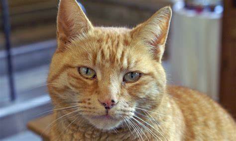
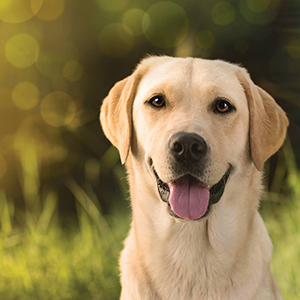
输出结果如下,不错吧:
Image path: BlogArchive/ml-08/cat.jpg
cat: 100.00%
dog: 0.00%
frog: 0.00%
deer: 0.00%
horse: 0.00%Image path: BlogArchive/ml-08/dog.jpg
dog: 100.00%
bird: 0.00%
deer: 0.00%
frog: 0.00%
horse: 0.00%
pytorch 有专门用于处理视觉信息的 torchvision,其中包含了 ResNet 的实现,也就是说其实我们不用自己去写🤒,如果你有兴趣可以参考里面的实现代码,再试试 ResNet-50 等层数更多的模型是否可以带来更好的效果。
1.5.使用CNN实现验证码识别(ResNet18)
最后再给出一个实用的例子。很多网站为了防机器人操作会使用验证码机制,传统的验证码会显示一张包含数字字母的图片,然后让用户填写里面的内容再对比是否正确,来判断用户是普通人还是机器人,这样的验证码可以用本篇介绍的 CNN 模型识别出来😈。
首先我们来选一个生成验证码的类库,github 上搜索 captcha c# 里面难度相对比较高的是 Hei.Captcha,这篇就使用 CNN 模型识别这个类库生成的验证码。(我的 zkweb 里面也有生成验证码的模块,但难度比较低所以就不用了)
以下步骤和代码会生成十万张用于训练和测试使用的验证码图片:
mkdir generate-captcha
cd generate-captcha
dotnet new console
dotnet add package Hei.Captcha
mkdir output
mkdir fonts
cd fonts
wget https://github.com/gebiWangshushu/Hei.Captcha/blob/master/Demo/fonts/Candara.ttf?raw=true
wget https://github.com/gebiWangshushu/Hei.Captcha/blob/master/Demo/fonts/STCAIYUN.ttf?raw=true
wget https://github.com/gebiWangshushu/Hei.Captcha/blob/master/Demo/fonts/impact.ttf?raw=true
wget https://github.com/gebiWangshushu/Hei.Captcha/blob/master/Demo/fonts/monbaiti.ttf?raw=true
cd ..
# 添加程序代码
dotnet run -c Release
using System;
using System.IO;
using Hei.Captcha;

namespace generate_captcha
{
    class Program
    {
        static void Main(string[] args)
        {
            var helper = new SecurityCodeHelper();
            var iterations = 100000;
            for (var x = 0; x < iterations; ++x)
            {
                var code = helper.GetRandomEnDigitalText(4);
                var bytes = helper.GetEnDigitalCodeByte(code);
                File.WriteAllBytes($"output/{x:D5}-{code}.png", bytes);
                if (x % 100 == 0)
                    Console.WriteLine($"{x}/{iterations}");
            }
        }
    }
}
以下是生成的验证码图片例子,变形旋转干扰线动态背景色该有的都有😠:


接下来我们想想应该用什么数据结构来表达验证码。在图片识别的例子中有十个分类,我们用了 onehot 编码,即使用长度为 10 的 tensor 对象来表示结果,正确的分类为 1,不正确的分类为 0。换成验证码以后,可以用长度为 36 的 tensor 对象来表示 1 位验证码 (26 个英文数字 + 10 个字母,假设验证码不分大小写),如果有多位则可以 36 * 位数的 tensor 对象来表达多位验证码。以下函数可以把验证码转换为对应的 tensor 对象:
# 字母数字列表
ALPHA_NUMS = "abcdefghijklmnopqrstuvwxyz0123456789"
ALPHA_NUMS_MAP = { c: index for index, c in enumerate(ALPHA_NUMS) }
# 验证码位数
DIGITS = 4
# 标签数量,字母数字混合*位数
NUM_LABELS = len(ALPHA_NUMS)*DIGITS

def code_to_tensor(code):
    """转换验证码到 tensor 对象,使用 onehot 编码"""
    t = torch.zeros((NUM_LABELS,))
    code = code.lower() # 验证码不分大小写
    for index, c in enumerate(code):
        p = ALPHA_NUMS_MAP[c]
        t[index*len(ALPHA_NUMS)+p] = 1
    return t
转换例子如下:
>>> code_to_tensor("abcd")
tensor([1., 0., 0., 0., 0., 0., 0., 0., 0., 0., 0., 0., 0., 0., 0., 0., 0., 0.,
        0., 0., 0., 0., 0., 0., 0., 0., 0., 0., 0., 0., 0., 0., 0., 0., 0., 0.,
        0., 1., 0., 0., 0., 0., 0., 0., 0., 0., 0., 0., 0., 0., 0., 0., 0., 0.,
        0., 0., 0., 0., 0., 0., 0., 0., 0., 0., 0., 0., 0., 0., 0., 0., 0., 0.,
        0., 0., 1., 0., 0., 0., 0., 0., 0., 0., 0., 0., 0., 0., 0., 0., 0., 0.,
        0., 0., 0., 0., 0., 0., 0., 0., 0., 0., 0., 0., 0., 0., 0., 0., 0., 0.,
        0., 0., 0., 1., 0., 0., 0., 0., 0., 0., 0., 0., 0., 0., 0., 0., 0., 0.,
        0., 0., 0., 0., 0., 0., 0., 0., 0., 0., 0., 0., 0., 0., 0., 0., 0., 0.])
>>> code_to_tensor("a123")
tensor([1., 0., 0., 0., 0., 0., 0., 0., 0., 0., 0., 0., 0., 0., 0., 0., 0., 0.,
        0., 0., 0., 0., 0., 0., 0., 0., 0., 0., 0., 0., 0., 0., 0., 0., 0., 0.,
        0., 0., 0., 0., 0., 0., 0., 0., 0., 0., 0., 0., 0., 0., 0., 0., 0., 0.,
        0., 0., 0., 0., 0., 0., 0., 0., 0., 1., 0., 0., 0., 0., 0., 0., 0., 0.,
        0., 0., 0., 0., 0., 0., 0., 0., 0., 0., 0., 0., 0., 0., 0., 0., 0., 0.,
        0., 0., 0., 0., 0., 0., 0., 0., 0., 0., 1., 0., 0., 0., 0., 0., 0., 0.,
        0., 0., 0., 0., 0., 0., 0., 0., 0., 0., 0., 0., 0., 0., 0., 0., 0., 0.,
        0., 0., 0., 0., 0., 0., 0., 0., 0., 0., 0., 1., 0., 0., 0., 0., 0., 0.])
反过来也一样,我们可以把 tensor 的长度按 36 分为多组,然后求每一组最大的值所在的索引,再根据该索引找到对应的字母或者数字,就可以把 tensor 对象转换回验证码:
def tensor_to_code(tensor):
    """转换 tensor 对象到验证码"""
    tensor = tensor.reshape(DIGITS, len(ALPHA_NUMS))
    indices = tensor.max(dim=1).indices
    code = "".join(ALPHA_NUMS[index] for index in indices)
    return code
接下来就可以用前面介绍过的 ResNet-18 模型进行训练了😎,相比前面的图片分类,这份代码有以下几点不同:
- 因为是多分类,损失计算器应该使用
BCELoss代替CrossEntropyLoss BCELoss要求模型输出值范围在 0 ~ 1 之间,所以需要在模型内部添加控制函数 (CrossEntropyLoss这么做会影响训练效果,但BCELoss不会)- 因为每一组都只有一个值是正确的,用
softmax效果会比sigmoid要好 (普通的多分类问题会使用sigmoid)
import os
import sys
import torch
import gzip
import itertools
import random
import numpy
import json
from PIL import Image
from torch import nn
from matplotlib import pyplot

# 分析目标的图片大小,全部图片都会先缩放到这个大小
# 验证码原图是 120x50
IMAGE_SIZE = (56, 24)
# 分析目标的图片所在的文件夹
IMAGE_DIR = "./generate-captcha/output/"
# 字母数字列表
ALPHA_NUMS = "abcdefghijklmnopqrstuvwxyz0123456789"
ALPHA_NUMS_MAP = { c: index for index, c in enumerate(ALPHA_NUMS) }
# 验证码位数
DIGITS = 4
# 标签数量,字母数字混合*位数
NUM_LABELS = len(ALPHA_NUMS)*DIGITS

class BasicBlock(nn.Module):
    """ResNet 使用的基础块"""
    expansion = 1 # 定义这个块的实际出通道是 channels_out 的几倍,这里的实现固定是一倍
    def __init__(self, channels_in, channels_out, stride):
        super().__init__()
        # 生成 3x3 的卷积层
        # 处理间隔 stride = 1 时,输出的长宽会等于输入的长宽,例如 (32-3+2)//1+1 == 32
        # 处理间隔 stride = 2 时,输出的长宽会等于输入的长宽的一半,例如 (32-3+2)//2+1 == 16
        # 此外 resnet 的 3x3 卷积层不使用偏移值 bias
        self.conv1 = nn.Sequential(
            nn.Conv2d(channels_in, channels_out, kernel_size=3, stride=stride, padding=1, bias=False),
            nn.BatchNorm2d(channels_out))
        # 再定义一个让输出和输入维度相同的 3x3 卷积层
        self.conv2 = nn.Sequential(
            nn.Conv2d(channels_out, channels_out, kernel_size=3, stride=1, padding=1, bias=False),
            nn.BatchNorm2d(channels_out))
        # 让原始输入和输出相加的时候,需要维度一致,如果维度不一致则需要整合
        self.identity = nn.Sequential()
        if stride != 1 or channels_in != channels_out * self.expansion:
            self.identity = nn.Sequential(
                nn.Conv2d(channels_in, channels_out * self.expansion, kernel_size=1, stride=stride, bias=False),
                nn.BatchNorm2d(channels_out * self.expansion))

    def forward(self, x):
        # x => conv1 => relu => conv2 => + => relu
        # |                              ^
        # |==============================|
        tmp = self.conv1(x)
        tmp = nn.functional.relu(tmp)
        tmp = self.conv2(tmp)
        tmp += self.identity(x)
        y = nn.functional.relu(tmp)
        return y

class MyModel(nn.Module):
    """识别验证码 (ResNet-18)"""
    def __init__(self, block_type = BasicBlock):
        super().__init__()
        # 记录上一层的出通道数量
        self.previous_channels_out = 64
        # 把 3 通道转换到 64 通道,长宽不变
        self.conv1 = nn.Sequential(
            nn.Conv2d(3, self.previous_channels_out, kernel_size=3, stride=1, padding=1, bias=False),
            nn.BatchNorm2d(self.previous_channels_out))
        # ResNet 使用的各个层
        self.layer1 = self._make_layer(block_type, channels_out=64, num_blocks=2, stride=1)
        self.layer2 = self._make_layer(block_type, channels_out=128, num_blocks=2, stride=2)
        self.layer3 = self._make_layer(block_type, channels_out=256, num_blocks=2, stride=2)
        self.layer4 = self._make_layer(block_type, channels_out=512, num_blocks=2, stride=2)
        # 把最后一层的长宽转换为 1x1 的池化层,Adaptive 表示会自动检测原有长宽
        # 例如 B,512,4,4 的矩阵会转换为 B,512,1,1,每个通道的单个值会是原有 16 个值的平均
        self.avgPool = nn.AdaptiveAvgPool2d((1, 1))
        # 全连接层,只使用单层线性模型
        self.fc_model = nn.Linear(512 * block_type.expansion, NUM_LABELS)
        # 控制输出在 0 ~ 1 之间,BCELoss 需要
        # 因为每组只应该有一个值为真,使用 softmax 效果会比 sigmoid 好
        self.softmax = nn.Softmax(dim=2)

    def _make_layer(self, block_type, channels_out, num_blocks, stride):
        blocks = []
        # 添加第一个块
        blocks.append(block_type(self.previous_channels_out, channels_out, stride))
        self.previous_channels_out = channels_out * block_type.expansion
        # 添加剩余的块,剩余的块固定处理间隔为 1,不会改变长宽
        for _ in range(num_blocks-1):
            blocks.append(block_type(self.previous_channels_out, self.previous_channels_out, 1))
            self.previous_channels_out *= block_type.expansion
        return nn.Sequential(*blocks)

    def forward(self, x):
        # 转换出通道到 64
        tmp = self.conv1(x)
        tmp = nn.functional.relu(tmp)
        # 应用 ResNet 的各个层
        tmp = self.layer1(tmp)
        tmp = self.layer2(tmp)
        tmp = self.layer3(tmp)
        tmp = self.layer4(tmp)
        # 转换长宽到 1x1
        tmp = self.avgPool(tmp)
        # 扁平化,维度会变为 B,512
        tmp = tmp.view(tmp.shape[0], -1)
        # 应用全连接层
        tmp = self.fc_model(tmp)
        # 划分每个字符对应的组,之后维度为 batch_size, digits, alpha_nums
        tmp = tmp.reshape(tmp.shape[0], DIGITS, len(ALPHA_NUMS))
        # 应用 softmax 到每一组
        tmp = self.softmax(tmp)
        # 重新扁平化,之后维度为 batch_size, num_labels
        y = tmp.reshape(tmp.shape[0], NUM_LABELS)
        return y

def save_tensor(tensor, path):
    """保存 tensor 对象到文件"""
    torch.save(tensor, gzip.GzipFile(path, "wb"))

def load_tensor(path):
    """从文件读取 tensor 对象"""
    return torch.load(gzip.GzipFile(path, "rb"))

def image_to_tensor(img):
    """转换图片对象到 tensor 对象"""
    in_img = img.resize(IMAGE_SIZE)
    in_img = in_img.convert("RGB") # 转换图片模式到 RGB
    arr = numpy.asarray(in_img)
    t = torch.from_numpy(arr)
    t = t.transpose(0, 2) # 转换维度 H,W,C 到 C,W,H
    t = t / 255.0 # 正规化数值使得范围在 0 ~ 1
    return t

def code_to_tensor(code):
    """转换验证码到 tensor 对象,使用 onehot 编码"""
    t = torch.zeros((NUM_LABELS,))
    code = code.lower() # 验证码不分大小写
    for index, c in enumerate(code):
        p = ALPHA_NUMS_MAP[c]
        t[index*len(ALPHA_NUMS)+p] = 1
    return t

def tensor_to_code(tensor):
    """转换 tensor 对象到验证码"""
    tensor = tensor.reshape(DIGITS, len(ALPHA_NUMS))
    indices = tensor.max(dim=1).indices
    code = "".join(ALPHA_NUMS[index] for index in indices)
    return code

def prepare_save_batch(batch, tensor_in, tensor_out):
    """准备训练 - 保存单个批次的数据"""
    # 切分训练集 (80%),验证集 (10%) 和测试集 (10%)
    random_indices = torch.randperm(tensor_in.shape[0])
    training_indices = random_indices[:int(len(random_indices)*0.8)]
    validating_indices = random_indices[int(len(random_indices)*0.8):int(len(random_indices)*0.9):]
    testing_indices = random_indices[int(len(random_indices)*0.9):]
    training_set = (tensor_in[training_indices], tensor_out[training_indices])
    validating_set = (tensor_in[validating_indices], tensor_out[validating_indices])
    testing_set = (tensor_in[testing_indices], tensor_out[testing_indices])

    # 保存到硬盘
    save_tensor(training_set, f"data/training_set.{batch}.pt")
    save_tensor(validating_set, f"data/validating_set.{batch}.pt")
    save_tensor(testing_set, f"data/testing_set.{batch}.pt")
    print(f"batch {batch} saved")

def prepare():
    """准备训练"""
    # 数据集转换到 tensor 以后会保存在 data 文件夹下
    if not os.path.isdir("data"):
        os.makedirs("data")

    # 查找所有图片
    image_paths = []
    for root, dirs, files in os.walk(IMAGE_DIR):
        for filename in files:
            path = os.path.join(root, filename)
            if not path.endswith(".png"):
                continue
            # 验证码在文件名中,例如
            # 00000-R865.png => R865
            code = filename.split(".")[0].split("-")[1]
            image_paths.append((path, code))

    # 打乱图片顺序
    random.shuffle(image_paths)

    # 分批读取和保存图片
    batch_size = 1000
    for batch in range(0, len(image_paths) // batch_size):
        image_tensors = []
        image_labels = []
        for path, code in image_paths[batch*batch_size:(batch+1)*batch_size]:
            with Image.open(path) as img:
                image_tensors.append(image_to_tensor(img))
            image_labels.append(code_to_tensor(code))
        tensor_in = torch.stack(image_tensors) # 维度: B,C,W,H
        tensor_out = torch.stack(image_labels) # 维度: B,N
        prepare_save_batch(batch, tensor_in, tensor_out)

def train():
    """开始训练"""
    # 创建模型实例
    model = MyModel()

    # 创建损失计算器
    # 计算多分类输出最好使用 BCELoss
    loss_function = torch.nn.BCELoss()

    # 创建参数调整器
    optimizer = torch.optim.Adam(model.parameters())

    # 记录训练集和验证集的正确率变化
    training_accuracy_history = []
    validating_accuracy_history = []

    # 记录最高的验证集正确率
    validating_accuracy_highest = -1
    validating_accuracy_highest_epoch = 0

    # 读取批次的工具函数
    def read_batches(base_path):
        for batch in itertools.count():
            path = f"{base_path}.{batch}.pt"
            if not os.path.isfile(path):
                break
            yield load_tensor(path)

    # 计算正确率的工具函数
    def calc_accuracy(actual, predicted):
        # 把每一位的最大值当作正确字符,然后比对有多少个字符相等
        actual_indices = actual.reshape(actual.shape[0], DIGITS, len(ALPHA_NUMS)).max(dim=2).indices
        predicted_indices = predicted.reshape(predicted.shape[0], DIGITS, len(ALPHA_NUMS)).max(dim=2).indices
        matched = (actual_indices - predicted_indices).abs().sum(dim=1) == 0
        acc = matched.sum().item() / actual.shape[0]
        return acc

    # 划分输入和输出的工具函数
    def split_batch_xy(batch, begin=None, end=None):
        # shape = batch_size, channels, width, height
        batch_x = batch[0][begin:end]
        # shape = batch_size, num_labels
        batch_y = batch[1][begin:end]
        return batch_x, batch_y

    # 开始训练过程
    for epoch in range(1, 10000):
        print(f"epoch: {epoch}")

        # 根据训练集训练并修改参数
        # 切换模型到训练模式,将会启用自动微分,批次正规化 (BatchNorm) 与 Dropout
        model.train()
        training_accuracy_list = []
        for batch_index, batch in enumerate(read_batches("data/training_set")):
            # 切分小批次,有助于泛化模型
            training_batch_accuracy_list = []
            for index in range(0, batch[0].shape[0], 100):
                # 划分输入和输出
                batch_x, batch_y = split_batch_xy(batch, index, index+100)
                # 计算预测值
                predicted = model(batch_x)
                # 计算损失
                loss = loss_function(predicted, batch_y)
                # 从损失自动微分求导函数值
                loss.backward()
                # 使用参数调整器调整参数
                optimizer.step()
                # 清空导函数值
                optimizer.zero_grad()
                # 记录这一个批次的正确率,torch.no_grad 代表临时禁用自动微分功能
                with torch.no_grad():
                    training_batch_accuracy_list.append(calc_accuracy(batch_y, predicted))
            # 输出批次正确率
            training_batch_accuracy = sum(training_batch_accuracy_list) / len(training_batch_accuracy_list)
            training_accuracy_list.append(training_batch_accuracy)
            print(f"epoch: {epoch}, batch: {batch_index}: batch accuracy: {training_batch_accuracy}")
        training_accuracy = sum(training_accuracy_list) / len(training_accuracy_list)
        training_accuracy_history.append(training_accuracy)
        print(f"training accuracy: {training_accuracy}")

        # 检查验证集
        # 切换模型到验证模式,将会禁用自动微分,批次正规化 (BatchNorm) 与 Dropout
        model.eval()
        validating_accuracy_list = []
        for batch in read_batches("data/validating_set"):
            batch_x, batch_y = split_batch_xy(batch)
            predicted = model(batch_x)
            validating_accuracy_list.append(calc_accuracy(batch_y, predicted))
        validating_accuracy = sum(validating_accuracy_list) / len(validating_accuracy_list)
        validating_accuracy_history.append(validating_accuracy)
        print(f"validating accuracy: {validating_accuracy}")

        # 记录最高的验证集正确率与当时的模型状态,判断是否在 20 次训练后仍然没有刷新记录
        if validating_accuracy > validating_accuracy_highest:
            validating_accuracy_highest = validating_accuracy
            validating_accuracy_highest_epoch = epoch
            save_tensor(model.state_dict(), "model.pt")
            print("highest validating accuracy updated")
        elif epoch - validating_accuracy_highest_epoch > 20:
            # 在 20 次训练后仍然没有刷新记录,结束训练
            print("stop training because highest validating accuracy not updated in 20 epoches")
            break

    # 使用达到最高正确率时的模型状态
    print(f"highest validating accuracy: {validating_accuracy_highest}",
        f"from epoch {validating_accuracy_highest_epoch}")
    model.load_state_dict(load_tensor("model.pt"))

    # 检查测试集
    testing_accuracy_list = []
    for batch in read_batches("data/testing_set"):
        batch_x, batch_y = split_batch_xy(batch)
        predicted = model(batch_x)
        testing_accuracy_list.append(calc_accuracy(batch_y, predicted))
    testing_accuracy = sum(testing_accuracy_list) / len(testing_accuracy_list)
    print(f"testing accuracy: {testing_accuracy}")

    # 显示训练集和验证集的正确率变化
    pyplot.plot(training_accuracy_history, label="training")
    pyplot.plot(validating_accuracy_history, label="validing")
    pyplot.ylim(0, 1)
    pyplot.legend()
    pyplot.show()

def eval_model():
    """使用训练好的模型"""
    # 创建模型实例,加载训练好的状态,然后切换到验证模式
    model = MyModel()
    model.load_state_dict(load_tensor("model.pt"))
    model.eval()

    # 询问图片路径,并显示可能的分类一览
    while True:
        try:
            # 构建输入
            image_path = input("Image path: ")
            if not image_path:
                continue
            with Image.open(image_path) as img:
                tensor_in = image_to_tensor(img).unsqueeze(0) # 维度 C,W,H => 1,C,W,H
            # 预测输出
            tensor_out = model(tensor_in)
            # 转换到验证码
            code = tensor_to_code(tensor_out[0])
            print(f"code: {code}")
            print()
        except Exception as e:
            print("error:", e)

def main():
    """主函数"""
    if len(sys.argv) < 2:
        print(f"Please run: {sys.argv[0]} prepare|train|eval")
        exit()

    # 给随机数生成器分配一个初始值,使得每次运行都可以生成相同的随机数
    # 这是为了让过程可重现,你也可以选择不这样做
    random.seed(0)
    torch.random.manual_seed(0)

    # 根据命令行参数选择操作
    operation = sys.argv[1]
    if operation == "prepare":
        prepare()
    elif operation == "train":
        train()
    elif operation == "eval":
        eval_model()
    else:
        raise ValueError(f"Unsupported operation: {operation}")

if __name__ == "__main__":
    main()
因为训练需要大量时间而我机器只有 CPU 可以用,所以这次我就只训练到 epoch 23 🤢,训练结果如下。可以看到训练集正确率达到了 98%,验证集正确率达到了 91%,已经是实用的级别了。
epoch: 23, batch: 98: batch accuracy: 0.99125
epoch: 23, batch: 99: batch accuracy: 0.9862500000000001
training accuracy: 0.9849874999999997
validating accuracy: 0.9103000000000003
highest validating accuracy updated
使用训练好的模型识别验证码,你可以对比上面的图片看看是不是识别对了 (第二张的 P 看起来很像 D 🤒):
$ python3 example.py eval
Image path: BlogArchive/ml-08/captcha-1.png
code: 8ca6

Image path: BlogArchive/ml-08/captcha-2.png
code: tp8s

Image path: BlogArchive/ml-08/captcha-3.png
code: k225
注意这里介绍出来的模型只能识别这一种验证码,其他不同种类的验证码需要分别训练和生成模型,做打码平台的话会先识别验证码种类再使用该种类对应的模型识别验证码内容。如果你的目标只是单种验证码,那么用这篇文章介绍的方法应该可以帮你节省调打码平台的钱 🤠。如果你机器有好显卡,也可以试试用更高级的模型提升正确率。
此外,有很多人问我现在流行的滑动验证码如何破解,其实破解这种验证码只需要做简单的图片分析,例如这里和这里都没有使用机器学习。但滑动验证码一般会配合浏览器指纹和鼠标轨迹采集一起使用,后台会根据大量数据分析用户是普通人还是机器人,所以破解几次很简单,但一直破解下去则会有很大几率被检测出来。
1.6.使用torchvision中的resnet模型
在前文我们看到了怎么组合卷积层和池化层自己实现 LeNet 和 ResNet-18,我们还可以使用 torchvision 中现成的模型,以下是修改识别验证码的模型到 torchvision 提供的 ResNet 实现的代码:
# 文件开头引用 torchvision 库
import torchvision

# 替换原有代码中的 MyModel 类,BasicBlock 可以删掉
class MyModel(nn.Module):
    """识别验证码 (ResNet-18)"""
    def __init__(self):
        super().__init__()
        # Resnet 的实现
        self.resnet = torchvision.models.resnet18(num_classes=NUM_LABELS)
        # 控制输出在 0 ~ 1 之间,BCELoss 需要
        # 因为每组只应该有一个值为真,使用 softmax 效果会比 sigmoid 好
        self.softmax = nn.Softmax(dim=2)

    def forward(self, x):
        # 应用 ResNet
        tmp = self.resnet(x)
        # 划分每个字符对应的组,之后维度为 batch_size, digits, alpha_nums
        tmp = tmp.reshape(tmp.shape[0], DIGITS, len(ALPHA_NUMS))
        # 应用 softmax 到每一组
        tmp = self.softmax(tmp)
        # 重新扁平化,之后维度为 batch_size, num_labels
        y = tmp.reshape(tmp.shape[0], NUM_LABELS)
        return y
是不是简单了很多?如果我们想使用 ResNet-50 可以把 resnet18 改为 resnet50 即可切换。虽然使用现成的模型方便,但了解下它们的原理和计算方式总是有好处的😇。
1.7.使用 GPU 训练识别验证码的模型
这里我拿前一篇文章的代码来展示怎样实际使用 GPU 训练识别验证码的模型,以下是修改后完整的代码:
如何生成训练数据和如何使用这份代码的说明请参考前一篇文章。
import os
import sys
import torch
import gzip
import itertools
import random
import numpy
import json
from PIL import Image
from torch import nn
from matplotlib import pyplot

# 分析目标的图片大小,全部图片都会先缩放到这个大小
# 验证码原图是 120x50
IMAGE_SIZE = (56, 24)
# 分析目标的图片所在的文件夹
IMAGE_DIR = "./generate-captcha/output/"
# 字母数字列表
ALPHA_NUMS = "abcdefghijklmnopqrstuvwxyz0123456789"
ALPHA_NUMS_MAP = { c: index for index, c in enumerate(ALPHA_NUMS) }
# 验证码位数
DIGITS = 4
# 标签数量,字母数字混合*位数
NUM_LABELS = len(ALPHA_NUMS)*DIGITS

# 用于启用 GPU 支持
device = torch.device("cuda" if torch.cuda.is_available() else "cpu")

class BasicBlock(nn.Module):
    """ResNet 使用的基础块"""
    expansion = 1 # 定义这个块的实际出通道是 channels_out 的几倍,这里的实现固定是一倍
    def __init__(self, channels_in, channels_out, stride):
        super().__init__()
        # 生成 3x3 的卷积层
        # 处理间隔 stride = 1 时,输出的长宽会等于输入的长宽,例如 (32-3+2)//1+1 == 32
        # 处理间隔 stride = 2 时,输出的长宽会等于输入的长宽的一半,例如 (32-3+2)//2+1 == 16
        # 此外 resnet 的 3x3 卷积层不使用偏移值 bias
        self.conv1 = nn.Sequential(
            nn.Conv2d(channels_in, channels_out, kernel_size=3, stride=stride, padding=1, bias=False),
            nn.BatchNorm2d(channels_out))
        # 再定义一个让输出和输入维度相同的 3x3 卷积层
        self.conv2 = nn.Sequential(
            nn.Conv2d(channels_out, channels_out, kernel_size=3, stride=1, padding=1, bias=False),
            nn.BatchNorm2d(channels_out))
        # 让原始输入和输出相加的时候,需要维度一致,如果维度不一致则需要整合
        self.identity = nn.Sequential()
        if stride != 1 or channels_in != channels_out * self.expansion:
            self.identity = nn.Sequential(
                nn.Conv2d(channels_in, channels_out * self.expansion, kernel_size=1, stride=stride, bias=False),
                nn.BatchNorm2d(channels_out * self.expansion))

    def forward(self, x):
        # x => conv1 => relu => conv2 => + => relu
        # |                              ^
        # |==============================|
        tmp = self.conv1(x)
        tmp = nn.functional.relu(tmp)
        tmp = self.conv2(tmp)
        tmp += self.identity(x)
        y = nn.functional.relu(tmp)
        return y

class MyModel(nn.Module):
    """识别验证码 (ResNet-18)"""
    def __init__(self, block_type = BasicBlock):
        super().__init__()
        # 记录上一层的出通道数量
        self.previous_channels_out = 64
        # 把 3 通道转换到 64 通道,长宽不变
        self.conv1 = nn.Sequential(
            nn.Conv2d(3, self.previous_channels_out, kernel_size=3, stride=1, padding=1, bias=False),
            nn.BatchNorm2d(self.previous_channels_out))
        # ResNet 使用的各个层
        self.layer1 = self._make_layer(block_type, channels_out=64, num_blocks=2, stride=1)
        self.layer2 = self._make_layer(block_type, channels_out=128, num_blocks=2, stride=2)
        self.layer3 = self._make_layer(block_type, channels_out=256, num_blocks=2, stride=2)
        self.layer4 = self._make_layer(block_type, channels_out=512, num_blocks=2, stride=2)
        # 把最后一层的长宽转换为 1x1 的池化层,Adaptive 表示会自动检测原有长宽
        # 例如 B,512,4,4 的矩阵会转换为 B,512,1,1,每个通道的单个值会是原有 16 个值的平均
        self.avgPool = nn.AdaptiveAvgPool2d((1, 1))
        # 全连接层,只使用单层线性模型
        self.fc_model = nn.Linear(512 * block_type.expansion, NUM_LABELS)
        # 控制输出在 0 ~ 1 之间,BCELoss 需要
        # 因为每组只应该有一个值为真,使用 softmax 效果会比 sigmoid 好
        self.softmax = nn.Softmax(dim=2)

    def _make_layer(self, block_type, channels_out, num_blocks, stride):
        blocks = []
        # 添加第一个块
        blocks.append(block_type(self.previous_channels_out, channels_out, stride))
        self.previous_channels_out = channels_out * block_type.expansion
        # 添加剩余的块,剩余的块固定处理间隔为 1,不会改变长宽
        for _ in range(num_blocks-1):
            blocks.append(block_type(self.previous_channels_out, self.previous_channels_out, 1))
            self.previous_channels_out *= block_type.expansion
        return nn.Sequential(*blocks)

    def forward(self, x):
        # 转换出通道到 64
        tmp = self.conv1(x)
        tmp = nn.functional.relu(tmp)
        # 应用 ResNet 的各个层
        tmp = self.layer1(tmp)
        tmp = self.layer2(tmp)
        tmp = self.layer3(tmp)
        tmp = self.layer4(tmp)
        # 转换长宽到 1x1
        tmp = self.avgPool(tmp)
        # 扁平化,维度会变为 B,512
        tmp = tmp.view(tmp.shape[0], -1)
        # 应用全连接层
        tmp = self.fc_model(tmp)
        # 划分每个字符对应的组,之后维度为 batch_size, digits, alpha_nums
        tmp = tmp.reshape(tmp.shape[0], DIGITS, len(ALPHA_NUMS))
        # 应用 softmax 到每一组
        tmp = self.softmax(tmp)
        # 重新扁平化,之后维度为 batch_size, num_labels
        y = tmp.reshape(tmp.shape[0], NUM_LABELS)
        return y

def save_tensor(tensor, path):
    """保存 tensor 对象到文件"""
    torch.save(tensor, gzip.GzipFile(path, "wb"))

def load_tensor(path):
    """从文件读取 tensor 对象"""
    return torch.load(gzip.GzipFile(path, "rb"))

def image_to_tensor(img):
    """转换图片对象到 tensor 对象"""
    in_img = img.resize(IMAGE_SIZE)
    in_img = in_img.convert("RGB") # 转换图片模式到 RGB
    arr = numpy.asarray(in_img)
    t = torch.from_numpy(arr)
    t = t.transpose(0, 2) # 转换维度 H,W,C 到 C,W,H
    t = t / 255.0 # 正规化数值使得范围在 0 ~ 1
    return t

def code_to_tensor(code):
    """转换验证码到 tensor 对象,使用 onehot 编码"""
    t = torch.zeros((NUM_LABELS,))
    code = code.lower() # 验证码不分大小写
    for index, c in enumerate(code):
        p = ALPHA_NUMS_MAP[c]
        t[index*len(ALPHA_NUMS)+p] = 1
    return t

def tensor_to_code(tensor):
    """转换 tensor 对象到验证码"""
    tensor = tensor.reshape(DIGITS, len(ALPHA_NUMS))
    indices = tensor.max(dim=1).indices
    code = "".join(ALPHA_NUMS[index] for index in indices)
    return code

def prepare_save_batch(batch, tensor_in, tensor_out):
    """准备训练 - 保存单个批次的数据"""
    # 切分训练集 (80%),验证集 (10%) 和测试集 (10%)
    random_indices = torch.randperm(tensor_in.shape[0])
    training_indices = random_indices[:int(len(random_indices)*0.8)]
    validating_indices = random_indices[int(len(random_indices)*0.8):int(len(random_indices)*0.9):]
    testing_indices = random_indices[int(len(random_indices)*0.9):]
    training_set = (tensor_in[training_indices], tensor_out[training_indices])
    validating_set = (tensor_in[validating_indices], tensor_out[validating_indices])
    testing_set = (tensor_in[testing_indices], tensor_out[testing_indices])

    # 保存到硬盘
    save_tensor(training_set, f"data/training_set.{batch}.pt")
    save_tensor(validating_set, f"data/validating_set.{batch}.pt")
    save_tensor(testing_set, f"data/testing_set.{batch}.pt")
    print(f"batch {batch} saved")

def prepare():
    """准备训练"""
    # 数据集转换到 tensor 以后会保存在 data 文件夹下
    if not os.path.isdir("data"):
        os.makedirs("data")

    # 查找所有图片
    image_paths = []
    for root, dirs, files in os.walk(IMAGE_DIR):
        for filename in files:
            path = os.path.join(root, filename)
            if not path.endswith(".png"):
                continue
            # 验证码在文件名中,例如
            # 00000-R865.png => R865
            code = filename.split(".")[0].split("-")[1]
            image_paths.append((path, code))

    # 打乱图片顺序
    random.shuffle(image_paths)

    # 分批读取和保存图片
    batch_size = 1000
    for batch in range(0, len(image_paths) // batch_size):
        image_tensors = []
        image_labels = []
        for path, code in image_paths[batch*batch_size:(batch+1)*batch_size]:
            with Image.open(path) as img:
                image_tensors.append(image_to_tensor(img))
            image_labels.append(code_to_tensor(code))
        tensor_in = torch.stack(image_tensors) # 维度: B,C,W,H
        tensor_out = torch.stack(image_labels) # 维度: B,N
        prepare_save_batch(batch, tensor_in, tensor_out)

def train():
    """开始训练"""
    # 创建模型实例
    model = MyModel().to(device)

    # 创建损失计算器
    # 计算多分类输出最好使用 BCELoss
    loss_function = torch.nn.BCELoss()

    # 创建参数调整器
    optimizer = torch.optim.Adam(model.parameters())

    # 记录训练集和验证集的正确率变化
    training_accuracy_history = []
    validating_accuracy_history = []

    # 记录最高的验证集正确率
    validating_accuracy_highest = -1
    validating_accuracy_highest_epoch = 0

    # 读取批次的工具函数
    def read_batches(base_path):
        for batch in itertools.count():
            path = f"{base_path}.{batch}.pt"
            if not os.path.isfile(path):
                break
            yield [ t.to(device) for t in load_tensor(path) ]

    # 计算正确率的工具函数
    def calc_accuracy(actual, predicted):
        # 把每一位的最大值当作正确字符,然后比对有多少个字符相等
        actual_indices = actual.reshape(actual.shape[0], DIGITS, len(ALPHA_NUMS)).max(dim=2).indices
        predicted_indices = predicted.reshape(predicted.shape[0], DIGITS, len(ALPHA_NUMS)).max(dim=2).indices
        matched = (actual_indices - predicted_indices).abs().sum(dim=1) == 0
        acc = matched.sum().item() / actual.shape[0]
        return acc

    # 划分输入和输出的工具函数
    def split_batch_xy(batch, begin=None, end=None):
        # shape = batch_size, channels, width, height
        batch_x = batch[0][begin:end]
        # shape = batch_size, num_labels
        batch_y = batch[1][begin:end]
        return batch_x, batch_y

    # 开始训练过程
    for epoch in range(1, 10000):
        print(f"epoch: {epoch}")

        # 根据训练集训练并修改参数
        # 切换模型到训练模式,将会启用自动微分,批次正规化 (BatchNorm) 与 Dropout
        model.train()
        training_accuracy_list = []
        for batch_index, batch in enumerate(read_batches("data/training_set")):
            # 切分小批次,有助于泛化模型
            training_batch_accuracy_list = []
            for index in range(0, batch[0].shape[0], 100):
                # 划分输入和输出
                batch_x, batch_y = split_batch_xy(batch, index, index+100)
                # 计算预测值
                predicted = model(batch_x)
                # 计算损失
                loss = loss_function(predicted, batch_y)
                # 从损失自动微分求导函数值
                loss.backward()
                # 使用参数调整器调整参数
                optimizer.step()
                # 清空导函数值
                optimizer.zero_grad()
                # 记录这一个批次的正确率,torch.no_grad 代表临时禁用自动微分功能
                with torch.no_grad():
                    training_batch_accuracy_list.append(calc_accuracy(batch_y, predicted))
            # 输出批次正确率
            training_batch_accuracy = sum(training_batch_accuracy_list) / len(training_batch_accuracy_list)
            training_accuracy_list.append(training_batch_accuracy)
            print(f"epoch: {epoch}, batch: {batch_index}: batch accuracy: {training_batch_accuracy}")
        training_accuracy = sum(training_accuracy_list) / len(training_accuracy_list)
        training_accuracy_history.append(training_accuracy)
        print(f"training accuracy: {training_accuracy}")

        # 检查验证集
        # 切换模型到验证模式,将会禁用自动微分,批次正规化 (BatchNorm) 与 Dropout
        model.eval()
        validating_accuracy_list = []
        for batch in read_batches("data/validating_set"):
            batch_x, batch_y = split_batch_xy(batch)
            predicted = model(batch_x)
            validating_accuracy_list.append(calc_accuracy(batch_y, predicted))
        validating_accuracy = sum(validating_accuracy_list) / len(validating_accuracy_list)
        validating_accuracy_history.append(validating_accuracy)
        print(f"validating accuracy: {validating_accuracy}")

        # 记录最高的验证集正确率与当时的模型状态,判断是否在 20 次训练后仍然没有刷新记录
        if validating_accuracy > validating_accuracy_highest:
            validating_accuracy_highest = validating_accuracy
            validating_accuracy_highest_epoch = epoch
            save_tensor(model.state_dict(), "model.pt")
            print("highest validating accuracy updated")
        elif epoch - validating_accuracy_highest_epoch > 20:
            # 在 20 次训练后仍然没有刷新记录,结束训练
            print("stop training because highest validating accuracy not updated in 20 epoches")
            break

    # 使用达到最高正确率时的模型状态
    print(f"highest validating accuracy: {validating_accuracy_highest}",
        f"from epoch {validating_accuracy_highest_epoch}")
    model.load_state_dict(load_tensor("model.pt"))

    # 检查测试集
    testing_accuracy_list = []
    for batch in read_batches("data/testing_set"):
        batch_x, batch_y = split_batch_xy(batch)
        predicted = model(batch_x)
        testing_accuracy_list.append(calc_accuracy(batch_y, predicted))
    testing_accuracy = sum(testing_accuracy_list) / len(testing_accuracy_list)
    print(f"testing accuracy: {testing_accuracy}")

    # 显示训练集和验证集的正确率变化
    pyplot.plot(training_accuracy_history, label="training")
    pyplot.plot(validating_accuracy_history, label="validing")
    pyplot.ylim(0, 1)
    pyplot.legend()
    pyplot.show()

def eval_model():
    """使用训练好的模型"""
    # 创建模型实例,加载训练好的状态,然后切换到验证模式
    model = MyModel().to(device)
    model.load_state_dict(load_tensor("model.pt"))
    model.eval()

    # 询问图片路径,并显示可能的分类一览
    while True:
        try:
            # 构建输入
            image_path = input("Image path: ")
            if not image_path:
                continue
            with Image.open(image_path) as img:
                tensor_in = image_to_tensor(img).to(device).unsqueeze(0) # 维度 C,W,H => 1,C,W,H
            # 预测输出
            tensor_out = model(tensor_in)
            # 转换到验证码
            code = tensor_to_code(tensor_out[0])
            print(f"code: {code}")
            print()
        except Exception as e:
            print("error:", e)

def main():
    """主函数"""
    if len(sys.argv) < 2:
        print(f"Please run: {sys.argv[0]} prepare|train|eval")
        exit()

    # 给随机数生成器分配一个初始值,使得每次运行都可以生成相同的随机数
    # 这是为了让过程可重现,你也可以选择不这样做
    random.seed(0)
    torch.random.manual_seed(0)

    # 根据命令行参数选择操作
    operation = sys.argv[1]
    if operation == "prepare":
        prepare()
    elif operation == "train":
        train()
    elif operation == "eval":
        eval_model()
    else:
        raise ValueError(f"Unsupported operation: {operation}")

if __name__ == "__main__":
    main()
使用 diff 生成相差的部分如下:
$ diff -U3 example.py.old example.py
@@ -23,6 +23,9 @@
 # 标签数量,字母数字混合*位数
 NUM_LABELS = len(ALPHA_NUMS)*DIGITS

+# 用于启用 GPU 支持
+device = torch.device("cuda" if torch.cuda.is_available() else "cpu")
+
 class BasicBlock(nn.Module):
     """ResNet 使用的基础块"""
     expansion = 1 # 定义这个块的实际出通道是 channels_out 的几倍,这里的实现固定是一倍
@@ -203,7 +206,7 @@
 def train():
     """开始训练"""
     # 创建模型实例
-    model = MyModel()
+    model = MyModel().to(device)

     # 创建损失计算器
     # 计算多分类输出最好使用 BCELoss
@@ -226,7 +229,7 @@
             path = f"{base_path}.{batch}.pt"
             if not os.path.isfile(path):
                 break
-            yield load_tensor(path)
+            yield [ t.to(device) for t in load_tensor(path) ]

     # 计算正确率的工具函数
     def calc_accuracy(actual, predicted):
@@ -327,7 +330,7 @@
 def eval_model():
     """使用训练好的模型"""
     # 创建模型实例,加载训练好的状态,然后切换到验证模式
-    model = MyModel()
+    model = MyModel().to(device)
     model.load_state_dict(load_tensor("model.pt"))
     model.eval()

@@ -339,7 +342,7 @@
             if not image_path:
                 continue
             with Image.open(image_path) as img:
-                tensor_in = image_to_tensor(img).unsqueeze(0) # 维度 C,W,H => 1,C,W,H
+                tensor_in = image_to_tensor(img).to(device).unsqueeze(0) # 维度 C,W,H => 1,C,W,H
             # 预测输出
             tensor_out = model(tensor_in)
             # 转换到验证码
可以看到只改动了五个部分,在头部添加了 device 的定义,然后在加载模型和 tensor 对象的时候使用 .to(device) 即可。
简单吧☺️。
那么训练速度相差如何呢?只训练一个 batch 使用 CPU 和 GPU 消耗的时间分别如下 (单位秒):
CPU: 13.60
GPU: 1.90
差了整整 7 倍😱,,如果是高端的显卡估计可以看到数十倍的差距。
1.8.显存占用
如果你想查看训练过程中的显存占用情况,可以使用 nvidia-smi 命令,命令会输出以下的信息:
+-----------------------------------------------------------------------------+
| NVIDIA-SMI 450.57       Driver Version: 450.57       CUDA Version: 11.0     |
|-------------------------------+----------------------+----------------------+
| GPU  Name        Persistence-M| Bus-Id        Disp.A | Volatile Uncorr. ECC |
| Fan  Temp  Perf  Pwr:Usage/Cap|         Memory-Usage | GPU-Util  Compute M. |
|                               |                      |               MIG M. |
|===============================+======================+======================|
|   0  GeForce GTX 1650    Off  | 00000000:06:00.0  On |                  N/A |
| 60%   67C    P3    40W /  90W |   3414MiB /  3902MiB |    100%      Default |
|                               |                      |                  N/A |
+-------------------------------+----------------------+----------------------+

+-----------------------------------------------------------------------------+
| Processes:                                                                  |
|  GPU   GI   CI        PID   Type   Process name                  GPU Memory |
|        ID   ID                                                   Usage      |
|=============================================================================|
|    0   N/A  N/A      1237      G   /usr/lib/xorg/Xorg                238MiB |
|    0   N/A  N/A      2545      G   cinnamon                           68MiB |
|    0   N/A  N/A      2797      G   ...AAAAAAAAA= --shared-files      103MiB |
|    0   N/A  N/A     18534      G   ...AAAAAAAAA= --shared-files       82MiB |
|    0   N/A  N/A     20035      C   python3                          2915MiB |
+-----------------------------------------------------------------------------+
如果训练过程中出现显存不足,你会看到以下的异常信息:
RuntimeError: CUDA error: out of memory
如果你遇到显存不足的问题,那么可以尝试以下的办法解决,按实用程度排序:
- 出钱买新显卡🤒
- 减少训练批次大小 (例如每个批次 100 条数据,减为每个批次 50 条数据)
- 不使用的对象早回收,例如
predicted = None,pytorch 会在对象声明周期结束后自动释放显存 - 计算单值的时候使用
item(),例如acc_total += acc.item(),但配合backward生成运算路径的计算不能用 - 如果你使用桌面 Linux,试试开机的时候添加
rw init=/bin/bash进入命令行界面再训练,这样可以节省个几百 MB 显存
你可能会好奇为什了 pytorch 可以及时释放显存,这是因为 python 的对象使用了引用计数 (Reference Counted),GC 基本上只负责回收循环引用的对象,对象的引用计数归 0 的时候 python 会自动调用析构函数,不需要等待 GC。而 NET 和 Java 等语言则无法做到及时回收,除非你每个 tensor 对象都及时的去调用 Dispose 方法,或者使用 tensorflow 来编译静态运算路径然后把生命周期管理工作全部交给框架。这也是使用 Python 的一大好处🥳。
二.对象识别RCNN与Fast-RCNN
2.1.图像分类与对象识别
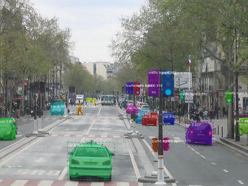
在前面的文章中我们看到了如何使用 CNN 模型识别图片里面的物体是什么类型,或者识别图片中固定的文字 (即验证码),因为模型会把整个图片当作输入并输出固定的结果,所以图片中只能有一个主要的物体或者固定数量的文字。
如果图片包含了多个物体,我们想识别有哪些物体,各个物体在什么位置,那么只用 CNN 模型是无法实现的。我们需要可以找出图片哪些区域包含物体并且判断每个区域包含什么物体的模型,这样的模型称为对象识别模型 (Object Detection Model),最早期的对象识别模型是 RCNN 模型,后来又发展出 Fast-RCNN (SPPnet),Faster-RCNN ,和 YOLO 等模型。因为对象识别需要处理的数据量多,速度会比较慢 (例如 RCNN 检测单张图片包含的物体可能需要几十秒),而对象识别通常又要求实时性 (例如来源是摄像头提供的视频),所以如何提升对象识别的速度是一个主要的命题,后面发展出的 Faster-RCNN 与 YOLO 都可以在一秒钟检测几十张图片。
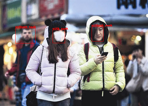
对象识别的应用范围比较广,例如人脸识别,车牌识别,自动驾驶等等都用到了对象识别的技术。对象识别是当今机器学习领域的一个前沿,2017 年研发出来的 Mask-RCNN 模型还可以检测对象的轮廓。
因为看上去越神奇的东西实现起来越难,对象识别模型相对于之前介绍的模型难度会高很多,请做好心理准备😱。
2.2.对象识别模型需要的训练数据
在介绍具体的模型之前,我们首先看看对象识别模型需要什么样的训练数据:
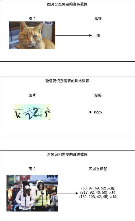
对象识别模型需要给每个图片标记有哪些区域,与每个区域对应的标签,也就是训练数据需要是列表形式的。区域的格式通常有两种,(x, y, w, h) => 左上角的坐标与长宽,与 (x1, y1, x2, y2) => 左上角与右下角的坐标,这两种格式可以互相转换,处理的时候只需要注意是哪种格式即可。标签除了需要识别的各个分类之外,还需要有一个特殊的非对象 (背景) 标签,表示这个区域不包含任何可以识别的对象,因为非对象区域通常可以自动生成,所以训练数据不需要包含非对象区域与标签。
2.3.RCNN
2.3.1.简介
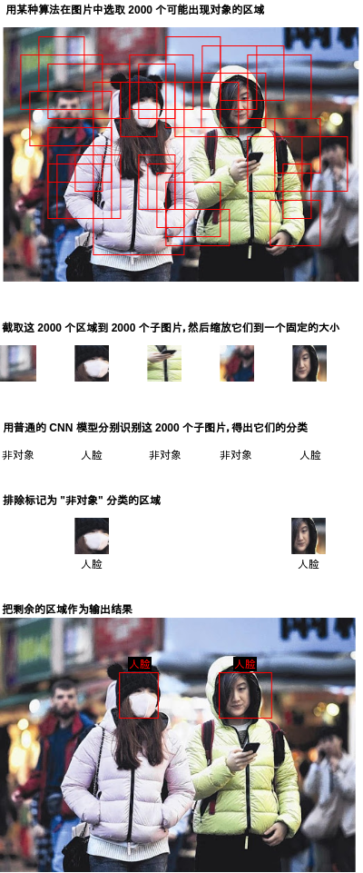
RCNN (Region Based Convolutional Neural Network) 是最早期的对象识别模型,实现比较简单,可以分为以下步骤:
- 用某种算法在图片中选取 2000 个可能出现对象的区域
- 截取这 2000 个区域到 2000 个子图片,然后缩放它们到一个固定的大小
- 用普通的 CNN 模型分别识别这 2000 个子图片,得出它们的分类
- 排除标记为 "非对象" 分类的区域
- 把剩余的区域作为输出结果
你可能已经从步骤里看出,RCNN 有几个大问题😠:
- 结果的精度很大程度取决于选取区域使用的算法
- 选取区域使用的算法是固定的,不参与学习,如果算法没有选出某个包含对象区域那么怎么学习都无法识别这个区域出来
- 慢,贼慢🐢,识别 1 张图片实际等于识别 2000 张图片
后面介绍模型结果会解决这些问题,但首先我们需要理解最简单的 RCNN 模型,接下来我们细看一下 RCNN 实现中几个重要的部分吧。
2.3.2.选取可能出现对象的区域
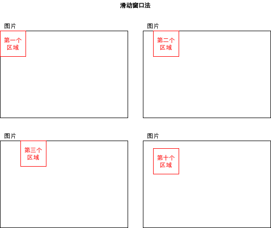
选取可能出现对象的区域的算法有很多种,例如滑动窗口法 (Sliding Window) 和选择性搜索法 (Selective Search)。滑动窗口法非常简单,决定一个固定大小的区域,然后按一定距离滑动得出下一个区域即可。滑动窗口法实现简单但选取出来的区域数量非常庞大并且精度很低,所以通常不会使用这种方法,除非物体大小固定并且出现的位置有一定规律。
选择性搜索法则比较高级,以下是简单的说明,摘自 opencv 的文章:
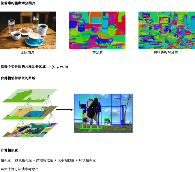
如果你觉得难以理解可以跳过,因为接下来我们会直接使用 opencv 类库中提供的选择搜索函数。而且选择搜索法精度也不高,后面介绍的模型将会使用更好的方法。
# 使用 opencv 类库中提供的选择搜索函数的代码例子
import cv2

img = cv2.imread("图片路径")
s = cv2.ximgproc.segmentation.createSelectiveSearchSegmentation()
s.setBaseImage(img)
s.switchToSelectiveSearchFast()
boxes = s.process() # 可能出现对象的所有区域,会按可能性排序
candidate_boxes = boxes[:2000] # 选取头 2000 个区域
2.3.3.按重叠率 (IOU) 判断每个区域是否包含对象
使用算法选取出来的区域与实际区域通常不会完全重叠,只会重叠一部分,在学习的过程中我们需要根据手头上的真实区域预先判断选取出来的区域是否包含对象,再告诉模型预测结果是否正确。判断选取区域是否包含对象会依据重叠率 (IOU - Intersection Over Union),所谓重叠率就是两个区域重叠的面积占两个区域合并的面积的比率,如下图所示。
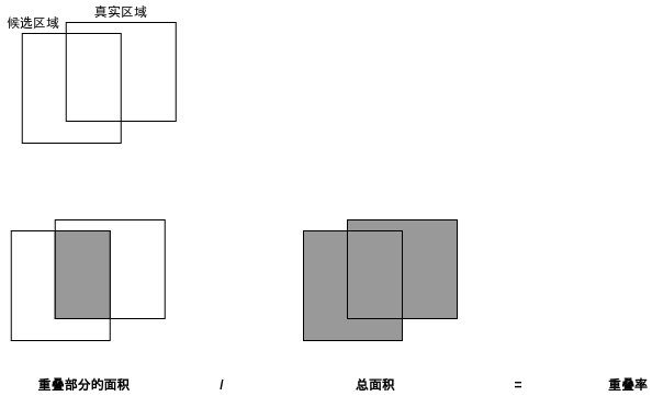
我们可以规定重叠率大于 70% 的候选区域包含对象,重叠率小于 30% 的区域不包含对象,而重叠率介于 30% ~ 70% 的区域不应该参与学习,这是为了给模型提供比较明确的数据,使得学习效果更好。
计算重叠率的代码如下,如果两个区域没有重叠则重叠率会为 0:
def calc_iou(rect1, rect2):
    """计算两个区域重叠部分 / 合并部分的比率 (intersection over union)"""
    x1, y1, w1, h1 = rect1
    x2, y2, w2, h2 = rect2
    xi = max(x1, x2)
    yi = max(y1, y2)
    wi = min(x1+w1, x2+w2) - xi
    hi = min(y1+h1, y2+h2) - yi
    if wi > 0 and hi > 0: # 有重叠部分
        area_overlap = wi*hi
        area_all = w1*h1 + w2*h2 - area_overlap
        iou = area_overlap / area_all
    else: # 没有重叠部分
        iou = 0
    return iou
原始论文
如果你想看 RCNN 的原始论文可以到以下的地址:
https://arxiv.org/pdf/1311.2524.pdf
2.4.使用RCNN识别图片中的人脸
好了,到这里你应该大致了解 RCNN 的实现原理,接下来我们试着用 RCNN 学习识别一些图片。
因为收集图片和标记图片非常累人🤕,为了偷懒这篇我还是使用现成的数据集。以下是包含人脸图片的数据集,并且带了各个人脸所在的区域的标记,格式是 (x1, y1, x2, y2)。下载需要注册帐号,但不需要交钱🤒。
Count the number of Faces present in an Image | Kaggle
下载解压后可以看到图片在 train/image_data 下,标记在 bbox_train.csv 中。
例如以下的图片:
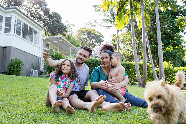
对应 csv 中的以下标记:
Name,width,height,xmin,ymin,xmax,ymax
10001.jpg,612,408,192,199,230,235
10001.jpg,612,408,247,168,291,211
10001.jpg,612,408,321,176,366,222
10001.jpg,612,408,355,183,387,214
数据的意义如下:
- Name: 文件名
- width: 图片整体宽度
- height: 图片整体高度
- xmin: 人脸区域的左上角的 x 坐标
- ymin: 人脸区域的左上角的 y 坐标
- xmax: 人脸区域的右下角的 x 坐标
- ymax: 人脸区域的右下角的 y 坐标
使用 RCNN 学习与识别这些图片中的人脸区域的代码如下:
import os
import sys
import torch
import gzip
import itertools
import random
import numpy
import pandas
import torchvision
import cv2
from torch import nn
from matplotlib import pyplot
from collections import defaultdict

# 各个区域缩放到的图片大小
REGION_IMAGE_SIZE = (32, 32)
# 分析目标的图片所在的文件夹
IMAGE_DIR = "./784145_1347673_bundle_archive/train/image_data"
# 定义各个图片中人脸区域的 CSV 文件
BOX_CSV_PATH = "./784145_1347673_bundle_archive/train/bbox_train.csv"

# 用于启用 GPU 支持
device = torch.device("cuda" if torch.cuda.is_available() else "cpu")

class MyModel(nn.Module):
    """识别是否人脸 (ResNet-18)"""
    def __init__(self):
        super().__init__()
        # Resnet 的实现
        # 输出两个分类 [非人脸, 人脸]
        self.resnet = torchvision.models.resnet18(num_classes=2)

    def forward(self, x):
        # 应用 ResNet
        y = self.resnet(x)
        return y

def save_tensor(tensor, path):
    """保存 tensor 对象到文件"""
    torch.save(tensor, gzip.GzipFile(path, "wb"))

def load_tensor(path):
    """从文件读取 tensor 对象"""
    return torch.load(gzip.GzipFile(path, "rb"))

def image_to_tensor(img):
    """转换 opencv 图片对象到 tensor 对象"""
    # 注意 opencv 是 BGR,但对训练没有影响所以不用转为 RGB
    img = cv2.resize(img, dsize=REGION_IMAGE_SIZE)
    arr = numpy.asarray(img)
    t = torch.from_numpy(arr)
    t = t.transpose(0, 2) # 转换维度 H,W,C 到 C,W,H
    t = t / 255.0 # 正规化数值使得范围在 0 ~ 1
    return t

def calc_iou(rect1, rect2):
    """计算两个区域重叠部分 / 合并部分的比率 (intersection over union)"""
    x1, y1, w1, h1 = rect1
    x2, y2, w2, h2 = rect2
    xi = max(x1, x2)
    yi = max(y1, y2)
    wi = min(x1+w1, x2+w2) - xi
    hi = min(y1+h1, y2+h2) - yi
    if wi > 0 and hi > 0: # 有重叠部分
        area_overlap = wi*hi
        area_all = w1*h1 + w2*h2 - area_overlap
        iou = area_overlap / area_all
    else: # 没有重叠部分
        iou = 0
    return iou

def selective_search(img):
    """计算 opencv 图片中可能出现对象的区域,只返回头 2000 个区域"""
    # 算法参考 https://www.learnopencv.com/selective-search-for-object-detection-cpp-python/
    s = cv2.ximgproc.segmentation.createSelectiveSearchSegmentation()
    s.setBaseImage(img)
    s.switchToSelectiveSearchFast()
    boxes = s.process()
    return boxes[:2000]

def prepare_save_batch(batch, image_tensors, image_labels):
    """准备训练 - 保存单个批次的数据"""
    # 生成输入和输出 tensor 对象
    tensor_in = torch.stack(image_tensors) # 维度: B,C,W,H
    tensor_out = torch.tensor(image_labels, dtype=torch.long) # 维度: B

    # 切分训练集 (80%),验证集 (10%) 和测试集 (10%)
    random_indices = torch.randperm(tensor_in.shape[0])
    training_indices = random_indices[:int(len(random_indices)*0.8)]
    validating_indices = random_indices[int(len(random_indices)*0.8):int(len(random_indices)*0.9):]
    testing_indices = random_indices[int(len(random_indices)*0.9):]
    training_set = (tensor_in[training_indices], tensor_out[training_indices])
    validating_set = (tensor_in[validating_indices], tensor_out[validating_indices])
    testing_set = (tensor_in[testing_indices], tensor_out[testing_indices])

    # 保存到硬盘
    save_tensor(training_set, f"data/training_set.{batch}.pt")
    save_tensor(validating_set, f"data/validating_set.{batch}.pt")
    save_tensor(testing_set, f"data/testing_set.{batch}.pt")
    print(f"batch {batch} saved")

def prepare():
    """准备训练"""
    # 数据集转换到 tensor 以后会保存在 data 文件夹下
    if not os.path.isdir("data"):
        os.makedirs("data")

    # 加载 csv 文件,构建图片到区域列表的索引 { 图片名: [ 区域, 区域, .. ] }
    box_map = defaultdict(lambda: [])
    df = pandas.read_csv(BOX_CSV_PATH)
    for row in df.values:
        filename, width, height, x1, y1, x2, y2 = row[:7]
        box_map[filename].append((x1, y1, x2-x1, y2-y1))

    # 从图片里面提取人脸 (正样本) 和非人脸 (负样本) 的图片
    batch_size = 1000
    batch = 0
    image_tensors = []
    image_labels = []
    for filename, true_boxes in box_map.items():
        path = os.path.join(IMAGE_DIR, filename)
        img = cv2.imread(path) # 加载原始图片
        candidate_boxes = selective_search(img) # 查找候选区域
        positive_samples = 0
        negative_samples = 0
        for candidate_box in candidate_boxes:
            # 如果候选区域和任意一个实际区域重叠率大于 70%,则认为是正样本
            # 如果候选区域和所有实际区域重叠率都小于 30%,则认为是负样本
            # 每个图片最多添加正样本数量 + 10 个负样本,需要提供足够多负样本避免伪阳性判断
            iou_list = [ calc_iou(candidate_box, true_box) for true_box in true_boxes ]
            positive_index = next((index for index, iou in enumerate(iou_list) if iou > 0.70), None)
            is_negative = all(iou < 0.30 for iou in iou_list)
            result = None
            if positive_index is not None:
                result = True
                positive_samples += 1
            elif is_negative and negative_samples < positive_samples + 10:
                result = False
                negative_samples += 1
            if result is not None:
                x, y, w, h = candidate_box
                child_img = img[y:y+h, x:x+w].copy()
                # 检验计算是否有问题
                # cv2.imwrite(f"{filename}_{x}_{y}_{w}_{h}_{int(result)}.png", child_img)
                image_tensors.append(image_to_tensor(child_img))
                image_labels.append(int(result))
                if len(image_tensors) >= batch_size:
                    # 保存批次
                    prepare_save_batch(batch, image_tensors, image_labels)
                    image_tensors.clear()
                    image_labels.clear()
                    batch += 1
    # 保存剩余的批次
    if len(image_tensors) > 10:
        prepare_save_batch(batch, image_tensors, image_labels)

def train():
    """开始训练"""
    # 创建模型实例
    model = MyModel().to(device)

    # 创建损失计算器
    loss_function = torch.nn.CrossEntropyLoss()

    # 创建参数调整器
    optimizer = torch.optim.Adam(model.parameters())

    # 记录训练集和验证集的正确率变化
    training_accuracy_history = []
    validating_accuracy_history = []

    # 记录最高的验证集正确率
    validating_accuracy_highest = -1
    validating_accuracy_highest_epoch = 0

    # 读取批次的工具函数
    def read_batches(base_path):
        for batch in itertools.count():
            path = f"{base_path}.{batch}.pt"
            if not os.path.isfile(path):
                break
            yield [ t.to(device) for t in load_tensor(path) ]

    # 计算正确率的工具函数,正样本和负样本的正确率分别计算再平均
    def calc_accuracy(actual, predicted):
        predicted = torch.max(predicted, 1).indices
        acc_positive = ((actual > 0.5) & (predicted > 0.5)).sum().item() / ((actual > 0.5).sum().item() + 0.00001)
        acc_negative = ((actual <= 0.5) & (predicted <= 0.5)).sum().item() / ((actual <= 0.5).sum().item() + 0.00001)
        acc = (acc_positive + acc_negative) / 2
        return acc

    # 划分输入和输出的工具函数
    def split_batch_xy(batch, begin=None, end=None):
        # shape = batch_size, channels, width, height
        batch_x = batch[0][begin:end]
        # shape = batch_size, num_labels
        batch_y = batch[1][begin:end]
        return batch_x, batch_y

    # 开始训练过程
    for epoch in range(1, 10000):
        print(f"epoch: {epoch}")

        # 根据训练集训练并修改参数
        model.train()
        training_accuracy_list = []
        for batch_index, batch in enumerate(read_batches("data/training_set")):
            # 切分小批次,有助于泛化模型
            training_batch_accuracy_list = []
            for index in range(0, batch[0].shape[0], 100):
                # 划分输入和输出
                batch_x, batch_y = split_batch_xy(batch, index, index+100)
                # 计算预测值
                predicted = model(batch_x)
                # 计算损失
                loss = loss_function(predicted, batch_y)
                # 从损失自动微分求导函数值
                loss.backward()
                # 使用参数调整器调整参数
                optimizer.step()
                # 清空导函数值
                optimizer.zero_grad()
                # 记录这一个批次的正确率,torch.no_grad 代表临时禁用自动微分功能
                with torch.no_grad():
                    training_batch_accuracy_list.append(calc_accuracy(batch_y, predicted))
            # 输出批次正确率
            training_batch_accuracy = sum(training_batch_accuracy_list) / len(training_batch_accuracy_list)
            training_accuracy_list.append(training_batch_accuracy)
            print(f"epoch: {epoch}, batch: {batch_index}: batch accuracy: {training_batch_accuracy}")
        training_accuracy = sum(training_accuracy_list) / len(training_accuracy_list)
        training_accuracy_history.append(training_accuracy)
        print(f"training accuracy: {training_accuracy}")

        # 检查验证集
        model.eval()
        validating_accuracy_list = []
        for batch in read_batches("data/validating_set"):
            batch_x, batch_y = split_batch_xy(batch)
            predicted = model(batch_x)
            validating_accuracy_list.append(calc_accuracy(batch_y, predicted))
        validating_accuracy = sum(validating_accuracy_list) / len(validating_accuracy_list)
        validating_accuracy_history.append(validating_accuracy)
        print(f"validating accuracy: {validating_accuracy}")

        # 记录最高的验证集正确率与当时的模型状态,判断是否在 20 次训练后仍然没有刷新记录
        if validating_accuracy > validating_accuracy_highest:
            validating_accuracy_highest = validating_accuracy
            validating_accuracy_highest_epoch = epoch
            save_tensor(model.state_dict(), "model.pt")
            print("highest validating accuracy updated")
        elif epoch - validating_accuracy_highest_epoch > 20:
            # 在 20 次训练后仍然没有刷新记录,结束训练
            print("stop training because highest validating accuracy not updated in 20 epoches")
            break

    # 使用达到最高正确率时的模型状态
    print(f"highest validating accuracy: {validating_accuracy_highest}",
        f"from epoch {validating_accuracy_highest_epoch}")
    model.load_state_dict(load_tensor("model.pt"))

    # 检查测试集
    testing_accuracy_list = []
    for batch in read_batches("data/testing_set"):
        batch_x, batch_y = split_batch_xy(batch)
        predicted = model(batch_x)
        testing_accuracy_list.append(calc_accuracy(batch_y, predicted))
    testing_accuracy = sum(testing_accuracy_list) / len(testing_accuracy_list)
    print(f"testing accuracy: {testing_accuracy}")

    # 显示训练集和验证集的正确率变化
    pyplot.plot(training_accuracy_history, label="training")
    pyplot.plot(validating_accuracy_history, label="validing")
    pyplot.ylim(0, 1)
    pyplot.legend()
    pyplot.show()

def eval_model():
    """使用训练好的模型"""
    # 创建模型实例,加载训练好的状态,然后切换到验证模式
    model = MyModel().to(device)
    model.load_state_dict(load_tensor("model.pt"))
    model.eval()

    # 询问图片路径,并显示所有可能是人脸的区域
    while True:
        try:
            # 选取可能出现对象的区域一览
            image_path = input("Image path: ")
            if not image_path:
                continue
            img = cv2.imread(image_path)
            candidate_boxes = selective_search(img)
            # 构建输入
            image_tensors = []
            for candidate_box in candidate_boxes:
                x, y, w, h = candidate_box
                child_img = img[y:y+h, x:x+w].copy()
                image_tensors.append(image_to_tensor(child_img))
            tensor_in = torch.stack(image_tensors).to(device)
            # 预测输出
            tensor_out = model(tensor_in)
            # 使用 softmax 计算是人脸的概率
            tensor_out = nn.functional.softmax(tensor_out, dim=1)
            tensor_out = tensor_out[:,1].resize(tensor_out.shape[0])
            # 判断概率大于 99% 的是人脸,添加边框到图片并保存
            img_output = img.copy()
            indices = torch.where(tensor_out > 0.99)[0]
            result_boxes = []
            result_boxes_all = []
            for index in indices:
                box = candidate_boxes[index]
                for exists_box in result_boxes_all:
                    # 如果和现存找到的区域重叠度大于 30% 则跳过
                    if calc_iou(exists_box, box) > 0.30:
                        break
                else:
                    result_boxes.append(box)
                result_boxes_all.append(box)
            for box in result_boxes:
                x, y, w, h = box
                print(x, y, w, h)
                cv2.rectangle(img_output, (x, y), (x+w, y+h), (0, 0, 0xff), 1)
            cv2.imwrite("img_output.png", img_output)
            print("saved to img_output.png")
            print()
        except Exception as e:
            print("error:", e)

def main():
    """主函数"""
    if len(sys.argv) < 2:
        print(f"Please run: {sys.argv[0]} prepare|train|eval")
        exit()

    # 给随机数生成器分配一个初始值,使得每次运行都可以生成相同的随机数
    # 这是为了让过程可重现,你也可以选择不这样做
    random.seed(0)
    torch.random.manual_seed(0)

    # 根据命令行参数选择操作
    operation = sys.argv[1]
    if operation == "prepare":
        prepare()
    elif operation == "train":
        train()
    elif operation == "eval":
        eval_model()
    else:
        raise ValueError(f"Unsupported operation: {operation}")

if __name__ == "__main__":
    main()
和之前文章给出的代码例子一样,这份代码也分为了 prepare, train, eval 三个部分,其中 prepare 部分负责选取区域,提取正样本 (包含人脸的区域) 和负样本 (不包含人脸的区域) 的子图片;train 使用普通的 resnet 模型学习子图片;eval 针对给出的图片选取区域并识别所有区域中是否包含人脸。
除了选取区域和提取子图片的处理以外,基本上和之前介绍的 CNN 模型一样吧🥳。
执行以下命令以后:
python3 example.py prepare
python3 example.py train
的最终输出如下:
epoch: 101, batch: 106: batch accuracy: 0.9999996838862198
epoch: 101, batch: 107: batch accuracy: 0.999218446914751
epoch: 101, batch: 108: batch accuracy: 0.9999996211125055
training accuracy: 0.999441394076678
validating accuracy: 0.9687856357743619
stop training because highest validating accuracy not updated in 20 epoches
highest validating accuracy: 0.9766918253771755 from epoch 80
testing accuracy: 0.9729761086851993
训练集和验证集的正确率变化如下:
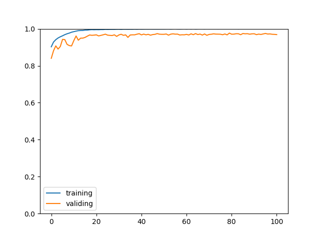
正确率看起来很高,但这只是针对选取后的区域判断的正确率,因为选取算法效果比较一般并且样本数量比较少,所以最终效果不能说令人满意😕。
执行以下命令,再输入图片路径可以使用学习好的模型识别图片:
python3 example.py eval
以下是部分识别结果:
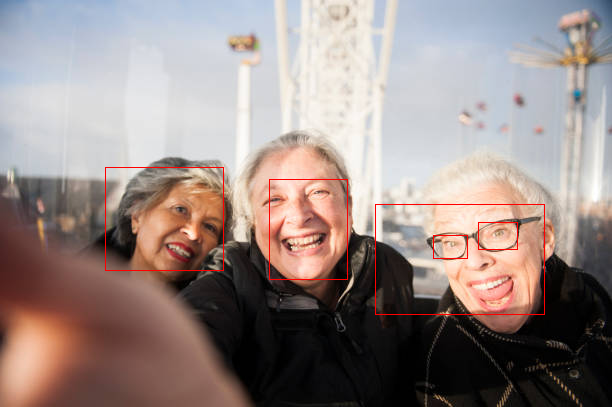
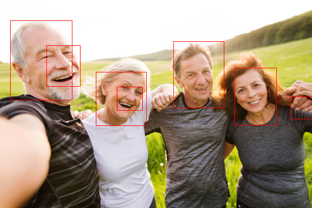
精度一般般😕。
2.5.Fast-RCNN
2.5.1.简介
RCNN 慢的原因主要是因为识别几千个子图片的计算量非常庞大,特别是这几千个子图片的范围很多是重合的,导致了很多重复的计算。Fast-RCNN 着重改善了这一部分,首先会针对整张图片生成一个与图片长宽相同 (或者等比例缩放) 的特征数据,然后再根据可能包含对象的区域截取特征数据,然后再根据截取后的子特征数据识别分类。RCNN 与 Fast-RCNN 的区别如下图所示:
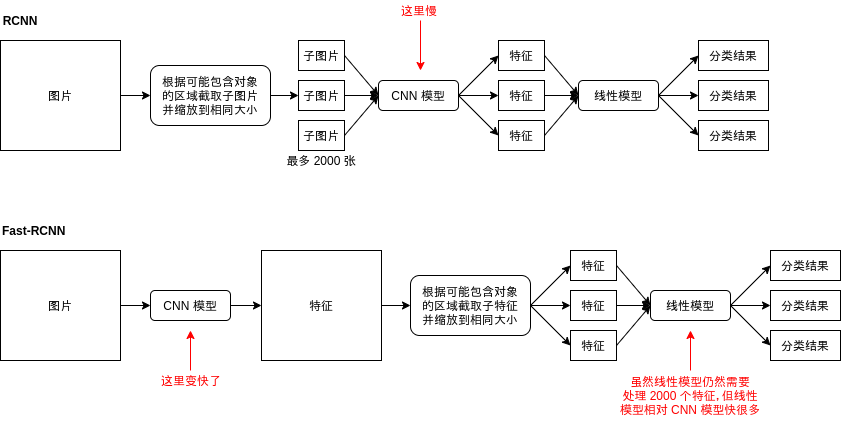
遗憾的是 Fast-RCNN 只是改善了速度,并不会改善正确率。但下面介绍的例子会引入一个比较重要的处理,即调整区域范围,它可以让模型给出的区域更接近实际的区域。
以下是 Fast-RCNN 模型中的一些处理细节。
2.5.2.缩放来源图片
在 RCNN 中,传给 CNN 模型的图片是经过缩放的子图片,而在 Fast-RCNN 中我们需要传原图片给 CNN 模型,那么原图片也需要进行缩放。缩放使用的方法是填充法,如下图所示:
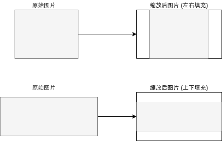
缩放图片使用的代码如下 (opencv 版):
IMAGE_SIZE = (128, 88)

def calc_resize_parameters(sw, sh):
    """计算缩放图片的参数"""
    sw_new, sh_new = sw, sh
    dw, dh = IMAGE_SIZE
    pad_w, pad_h = 0, 0
    if sw / sh < dw / dh:
        sw_new = int(dw / dh * sh)
        pad_w = (sw_new - sw) // 2 # 填充左右
    else:
        sh_new = int(dh / dw * sw)
        pad_h = (sh_new - sh) // 2 # 填充上下
    return sw_new, sh_new, pad_w, pad_h

def resize_image(img):
    """缩放 opencv 图片,比例不一致时填充"""
    sh, sw, _ = img.shape
    sw_new, sh_new, pad_w, pad_h = calc_resize_parameters(sw, sh)
    img = cv2.copyMakeBorder(img, pad_h, pad_h, pad_w, pad_w, cv2.BORDER_CONSTANT, (0, 0, 0))
    img = cv2.resize(img, dsize=IMAGE_SIZE)
    return img
缩放图片后区域的坐标也需要转换,转换的代码如下 (都是枯燥的代码🤒):
IMAGE_SIZE = (128, 88)

def map_box_to_resized_image(box, sw, sh):
    """把原始区域转换到缩放后的图片对应的区域"""
    x, y, w, h = box
    sw_new, sh_new, pad_w, pad_h = calc_resize_parameters(sw, sh)
    scale = IMAGE_SIZE[0] / sw_new
    x = int((x + pad_w) * scale)
    y = int((y + pad_h) * scale)
    w = int(w * scale)
    h = int(h * scale)
    if x + w > IMAGE_SIZE[0] or y + h > IMAGE_SIZE[1] or w == 0 or h == 0:
        return 0, 0, 0, 0
    return x, y, w, h

def map_box_to_original_image(box, sw, sh):
    """把缩放后图片对应的区域转换到缩放前的原始区域"""
    x, y, w, h = box
    sw_new, sh_new, pad_w, pad_h = calc_resize_parameters(sw, sh)
    scale = IMAGE_SIZE[0] / sw_new
    x = int(x / scale - pad_w)
    y = int(y / scale - pad_h)
    w = int(w / scale)
    h = int(h / scale)
    if x + w > sw or y + h > sh or x < 0 or y < 0 or w == 0 or h == 0:
        return 0, 0, 0, 0
    return x, y, w, h
2.5.3.计算区域特征
在前面的文章中我们已经了解过,CNN 模型可以分为卷积层,池化层和全连接层,卷积层,池化层用于抽取图片中各个区域的特征,全连接层用于把特征扁平化并交给线性模型处理。在 Fast-RCNN 中,我们不需要使用整张图片的特征,只需要使用部分区域的特征,所以 Fast-RCNN 使用的 CNN 模型只需要卷积层和池化层 (部分模型池化层可以省略),卷积层输出的通道数量通常会比图片原有的通道数量多,并且长宽会按原来图片的长宽等比例缩小,例如原图的大小是 3,256,256 的时候,经过处理可能会输出 512,32,32,代表每个 8x8 像素的区域都对应 512 个特征。
这篇给出的 Fast-RCN 代码为了易于理解,会让 CNN 模型输出和原图一模一样的大小,这样抽取区域特征的时候只需要使用 [] 操作符即可。
2.5.4.抽取区域特征(ROI Pooling)
Fast-RCNN 根据整张图片生成特征以后,下一步就是抽取区域特征 (Region of interest Pooling) 了,抽取区域特征简单的来说就是根据区域在图片中的位置,截区域中该位置的数据,然后再缩放到相同大小,如下图所示:
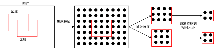
抽取区域特征的层又称为 ROI 层。
如果特征的长宽和图片的长宽相同,那么截取特征只需要简单的 [] 操作,但如果特征的长宽比图片的长宽要小,那么就需要使用近邻插值法 (Nearest Neighbor Interpolation) 或者双线插值法 (Bilinear Interpolation) 进行截取,使用双线插值法进行截取的 ROI 层又称作 ROI Align。截取以后的缩放可以使用 MaxPool,近邻插值法或双线插值法等算法。
想更好的理解 ROI Align 与双线插值法可以参考这篇文章。
2.5.5.调整区域范围
在前面已经提到过,使用选择搜索法等算法选取出来的区域与对象实际所在的区域可能有一定偏差,这个偏差是可以通过模型来调整的。举个简单的例子,如果区域内有脸的左半部分,那么模型在经过学习后应该可以判断出区域应该向右扩展一些。
区域调整可以分为四个参数:
- 对左上角 x 坐标的调整
- 对左上角 y 坐标的调整
- 对长度的调整
- 对宽度的调整
因为坐标和长宽的值大小不一定,例如同样是脸的左半部分,出现在图片的左上角和图片的右下角就会让 x y 坐标不一样,如果远近不同那么长宽也会不一样,我们需要把调整量作标准化,标准化的公式如下:
- x1, y1, w1, h1 = 候选区域
- x2, y2, w2, h2 = 真实区域
- x 偏移 = (x2 - x1) / w1
- y 偏移 = (y2 - y1) / h1
- w 偏移 = log(w2 / w1)
- h 偏移 = log(h2 / h1)
经过标准化后,偏移的值就会作为比例而不是绝对值,不会受具体坐标和长宽的影响。此外,公式中使用 log 是为了减少偏移的增幅,使得偏移比较大的时候模型仍然可以达到比较好的学习效果。
计算区域调整偏移和根据偏移调整区域的代码如下:
def calc_box_offset(candidate_box, true_box):
    """计算候选区域与实际区域的偏移值"""
    x1, y1, w1, h1 = candidate_box
    x2, y2, w2, h2 = true_box
    x_offset = (x2 - x1) / w1
    y_offset = (y2 - y1) / h1
    w_offset = math.log(w2 / w1)
    h_offset = math.log(h2 / h1)
    return (x_offset, y_offset, w_offset, h_offset)

def adjust_box_by_offset(candidate_box, offset):
    """根据偏移值调整候选区域"""
    x1, y1, w1, h1 = candidate_box
    x_offset, y_offset, w_offset, h_offset = offset
    x2 = w1 * x_offset + x1
    y2 = h1 * y_offset + y1
    w2 = math.exp(w_offset) * w1
    h2 = math.exp(h_offset) * h1
    return (x2, y2, w2, h2)
2.5.6.计算损失
Fast-RCNN 模型会针对各个区域输出两个结果,第一个是区域对应的标签 (人脸,非人脸),第二个是上面提到的区域偏移,调整参数的时候也需要同时根据这两个结果调整。实现同时调整多个结果可以把损失相加起来再计算各个参数的导函数值:
各个区域的特征 = ROI层(CNN模型(图片数据))
计算标签的线性模型(各个区域的特征) - 真实标签 = 标签损失
计算偏移的线性模型(各个区域的特征) - 真实偏移 = 偏移损失损失 = 标签损失 + 偏移损失
有一个需要注意的地方是,在这个例子里计算标签损失需要分别根据正负样本计算,否则模型在经过调整以后只会输出负结果。这是因为线性模型计算抽取出来的特征时有可能输出正 (人脸),也有可能输出负 (非人脸),而 ROI 层抽取的特征很多是重合的,也就是来源相同,当负样本比正样本要多的时候,结果的方向就会更偏向于负,这样每次调整参数的时候都会向输出负的方向调整。如果把损失分开计算,那么不重合的特征可以分别向输出正负的方向调整,从而达到学习的效果。
此外,偏移损失只应该根据正样本计算,负样本没有必要学习偏移。
最终的损失计算处理如下:
各个区域的特征 = ROI层(CNN模型(图片数据))
计算标签的线性模型(各个区域的特征)[正样本] - 真实标签[正样本] = 正样本标签损失
计算标签的线性模型(各个区域的特征)[负样本] - 真实标签[负样本] = 负样本标签损失
计算偏移的线性模型(各个区域的特征)[正样本] - 真实偏移[正样本] = 正样本偏移损失损失 = 正样本标签损失 + 负样本标签损失 + 正样本偏移损失
2.5.7.合并结果区域
因为选取区域的算法本来就会返回很多重合的区域,可能会有有好几个区域同时和真实区域重叠率大于一定值 (70%),导致这几个区域都会被认为是包含对象的区域:
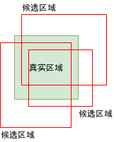
模型经过学习后,针对图片预测得出结果时也有可能返回这样的重合区域,合并这样的区域有几种方法:
- 使用最左,最右,最上,或者最下的区域
- 使用第一个区域 (区域选取算法会按出现对象的可能性排序)
- 结合所有重合的区域 (如果区域调整效果不行,则可能出现结果区域比真实区域大很多的问题)
上面给出的 RCNN 代码例子已经使用第二个方法合并结果区域,下面给出的例子也会使用同样的方法。但下一篇文章的 Faster-RCNN 则会使用第三个方法,因为 Faster-RCNN 的区域调整效果相对比较好。
2.5.8.原始论文
如果你想看 Fast-RCNN 的原始论文可以到以下的地址:
https://arxiv.org/pdf/1504.08083.pdf
2.6.使用Fast-RCNN识别图片中的人脸
代码时间到了😱,这份代码会使用 Fast-RCNN 模型来图片中的人脸,使用的数据集和前面的例子一样。
import os
import sys
import torch
import gzip
import itertools
import random
import numpy
import math
import pandas
import cv2
from torch import nn
from matplotlib import pyplot
from collections import defaultdict

# 缩放图片的大小
IMAGE_SIZE = (256, 256)
# 分析目标的图片所在的文件夹
IMAGE_DIR = "./784145_1347673_bundle_archive/train/image_data"
# 定义各个图片中人脸区域的 CSV 文件
BOX_CSV_PATH = "./784145_1347673_bundle_archive/train/bbox_train.csv"

# 用于启用 GPU 支持
device = torch.device("cuda" if torch.cuda.is_available() else "cpu")

class BasicBlock(nn.Module):
    """ResNet 使用的基础块"""
    expansion = 1 # 定义这个块的实际出通道是 channels_out 的几倍,这里的实现固定是一倍
    def __init__(self, channels_in, channels_out, stride):
        super().__init__()
        # 生成 3x3 的卷积层
        # 处理间隔 stride = 1 时,输出的长宽会等于输入的长宽,例如 (32-3+2)//1+1 == 32
        # 处理间隔 stride = 2 时,输出的长宽会等于输入的长宽的一半,例如 (32-3+2)//2+1 == 16
        # 此外 resnet 的 3x3 卷积层不使用偏移值 bias
        self.conv1 = nn.Sequential(
            nn.Conv2d(channels_in, channels_out, kernel_size=3, stride=stride, padding=1, bias=False),
            nn.BatchNorm2d(channels_out))
        # 再定义一个让输出和输入维度相同的 3x3 卷积层
        self.conv2 = nn.Sequential(
            nn.Conv2d(channels_out, channels_out, kernel_size=3, stride=1, padding=1, bias=False),
            nn.BatchNorm2d(channels_out))
        # 让原始输入和输出相加的时候,需要维度一致,如果维度不一致则需要整合
        self.identity = nn.Sequential()
        if stride != 1 or channels_in != channels_out * self.expansion:
            self.identity = nn.Sequential(
                nn.Conv2d(channels_in, channels_out * self.expansion, kernel_size=1, stride=stride, bias=False),
                nn.BatchNorm2d(channels_out * self.expansion))

    def forward(self, x):
        # x => conv1 => relu => conv2 => + => relu
        # |                              ^
        # |==============================|
        tmp = self.conv1(x)
        tmp = nn.functional.relu(tmp, inplace=True)
        tmp = self.conv2(tmp)
        tmp += self.identity(x)
        y = nn.functional.relu(tmp, inplace=True)
        return y

class MyModel(nn.Module):
    """Fast-RCNN (基于 ResNet-18 的变种)"""
    def __init__(self):
        super().__init__()
        # 记录上一层的出通道数量
        self.previous_channels_out = 4
        # 把 3 通道转换到 4 通道,长宽不变
        self.conv1 = nn.Sequential(
            nn.Conv2d(3, self.previous_channels_out, kernel_size=3, stride=1, padding=1, bias=False),
            nn.BatchNorm2d(self.previous_channels_out))
        # 抽取图片各个区域特征的 ResNet (除去 AvgPool 和全连接层)
        # 和原始的 Resnet 不一样的是输出的长宽和输入的长宽会相等,以便 ROI 层按区域抽取R征
        # 此外,为了可以让模型跑在 4GB 显存上,这里减少了模型的通道数量
        self.layer1 = self._make_layer(BasicBlock, channels_out=4, num_blocks=2, stride=1)
        self.layer2 = self._make_layer(BasicBlock, channels_out=4, num_blocks=2, stride=1)
        self.layer3 = self._make_layer(BasicBlock, channels_out=8, num_blocks=2, stride=1)
        self.layer4 = self._make_layer(BasicBlock, channels_out=8, num_blocks=2, stride=1)
        # ROI 层抽取各个子区域特征后转换到固定大小
        self.roi_pool = nn.AdaptiveMaxPool2d((5, 5))
        # 输出两个分类 [非人脸, 人脸]
        self.fc_labels_model = nn.Sequential(
            nn.Linear(8*5*5, 32),
            nn.ReLU(),
            nn.Dropout(0.1),
            nn.Linear(32, 2))
        # 计算区域偏移,分别输出 x, y, w, h 的偏移
        self.fc_offsets_model = nn.Sequential(
            nn.Linear(8*5*5, 128),
            nn.ReLU(),
            nn.Dropout(0.1),
            nn.Linear(128, 4))

    def _make_layer(self, block_type, channels_out, num_blocks, stride):
        blocks = []
        # 添加第一个块
        blocks.append(block_type(self.previous_channels_out, channels_out, stride))
        self.previous_channels_out = channels_out * block_type.expansion
        # 添加剩余的块,剩余的块固定处理间隔为 1,不会改变长宽
        for _ in range(num_blocks-1):
            blocks.append(block_type(self.previous_channels_out, self.previous_channels_out, 1))
            self.previous_channels_out *= block_type.expansion
        return nn.Sequential(*blocks)

    def _roi_pooling(self, feature_mapping, roi_boxes):
        result = []
        for box in roi_boxes:
            image_index, x, y, w, h = map(int, box.tolist())
            feature_sub_region = feature_mapping[image_index][:,x:x+w,y:y+h]
            fixed_features = self.roi_pool(feature_sub_region).reshape(-1) # 顺道扁平化
            result.append(fixed_features)
        return torch.stack(result)

    def forward(self, x):
        images_tensor = x[0]
        candidate_boxes_tensor = x[1]
        # 转换出通道
        tmp = self.conv1(images_tensor)
        tmp = nn.functional.relu(tmp)
        # 应用 ResNet 的各个层
        # 结果维度是 B,32,W,H
        tmp = self.layer1(tmp)
        tmp = self.layer2(tmp)
        tmp = self.layer3(tmp)
        tmp = self.layer4(tmp)
        # 使用 ROI 层抽取各个子区域的特征并转换到固定大小
        # 结果维度是 B,32*9*9
        tmp = self._roi_pooling(tmp, candidate_boxes_tensor)
        # 根据抽取出来的子区域特征分别计算分类 (是否人脸) 和区域偏移
        labels = self.fc_labels_model(tmp)
        offsets = self.fc_offsets_model(tmp)
        y = (labels, offsets)
        return y

def save_tensor(tensor, path):
    """保存 tensor 对象到文件"""
    torch.save(tensor, gzip.GzipFile(path, "wb"))

def load_tensor(path):
    """从文件读取 tensor 对象"""
    return torch.load(gzip.GzipFile(path, "rb"))

def calc_resize_parameters(sw, sh):
    """计算缩放图片的参数"""
    sw_new, sh_new = sw, sh
    dw, dh = IMAGE_SIZE
    pad_w, pad_h = 0, 0
    if sw / sh < dw / dh:
        sw_new = int(dw / dh * sh)
        pad_w = (sw_new - sw) // 2 # 填充左右
    else:
        sh_new = int(dh / dw * sw)
        pad_h = (sh_new - sh) // 2 # 填充上下
    return sw_new, sh_new, pad_w, pad_h

def resize_image(img):
    """缩放 opencv 图片,比例不一致时填充"""
    sh, sw, _ = img.shape
    sw_new, sh_new, pad_w, pad_h = calc_resize_parameters(sw, sh)
    img = cv2.copyMakeBorder(img, pad_h, pad_h, pad_w, pad_w, cv2.BORDER_CONSTANT, (0, 0, 0))
    img = cv2.resize(img, dsize=IMAGE_SIZE)
    return img

def image_to_tensor(img):
    """转换 opencv 图片对象到 tensor 对象"""
    # 注意 opencv 是 BGR,但对训练没有影响所以不用转为 RGB
    arr = numpy.asarray(img)
    t = torch.from_numpy(arr)
    t = t.transpose(0, 2) # 转换维度 H,W,C 到 C,W,H
    t = t / 255.0 # 正规化数值使得范围在 0 ~ 1
    return t

def map_box_to_resized_image(box, sw, sh):
    """把原始区域转换到缩放后的图片对应的区域"""
    x, y, w, h = box
    sw_new, sh_new, pad_w, pad_h = calc_resize_parameters(sw, sh)
    scale = IMAGE_SIZE[0] / sw_new
    x = int((x + pad_w) * scale)
    y = int((y + pad_h) * scale)
    w = int(w * scale)
    h = int(h * scale)
    if x + w > IMAGE_SIZE[0] or y + h > IMAGE_SIZE[1] or w == 0 or h == 0:
        return 0, 0, 0, 0
    return x, y, w, h

def map_box_to_original_image(box, sw, sh):
    """把缩放后图片对应的区域转换到缩放前的原始区域"""
    x, y, w, h = box
    sw_new, sh_new, pad_w, pad_h = calc_resize_parameters(sw, sh)
    scale = IMAGE_SIZE[0] / sw_new
    x = int(x / scale - pad_w)
    y = int(y / scale - pad_h)
    w = int(w / scale)
    h = int(h / scale)
    if x + w > sw or y + h > sh or x < 0 or y < 0 or w == 0 or h == 0:
        return 0, 0, 0, 0
    return x, y, w, h

def calc_iou(rect1, rect2):
    """计算两个区域重叠部分 / 合并部分的比率 (intersection over union)"""
    x1, y1, w1, h1 = rect1
    x2, y2, w2, h2 = rect2
    xi = max(x1, x2)
    yi = max(y1, y2)
    wi = min(x1+w1, x2+w2) - xi
    hi = min(y1+h1, y2+h2) - yi
    if wi > 0 and hi > 0: # 有重叠部分
        area_overlap = wi*hi
        area_all = w1*h1 + w2*h2 - area_overlap
        iou = area_overlap / area_all
    else: # 没有重叠部分
        iou = 0
    return iou

def calc_box_offset(candidate_box, true_box):
    """计算候选区域与实际区域的偏移值"""
    # 这里计算出来的偏移值基于比例,而不受具体位置和大小影响
    # w h 使用 log 是为了减少过大的值的影响
    x1, y1, w1, h1 = candidate_box
    x2, y2, w2, h2 = true_box
    x_offset = (x2 - x1) / w1
    y_offset = (y2 - y1) / h1
    w_offset = math.log(w2 / w1)
    h_offset = math.log(h2 / h1)
    return (x_offset, y_offset, w_offset, h_offset)

def adjust_box_by_offset(candidate_box, offset):
    """根据偏移值调整候选区域"""
    x1, y1, w1, h1 = candidate_box
    x_offset, y_offset, w_offset, h_offset = offset
    x2 = w1 * x_offset + x1
    y2 = h1 * y_offset + y1
    w2 = math.exp(w_offset) * w1
    h2 = math.exp(h_offset) * h1
    return (x2, y2, w2, h2)

def selective_search(img):
    """计算 opencv 图片中可能出现对象的区域,只返回头 2000 个区域"""
    # 算法参考 https://www.learnopencv.com/selective-search-for-object-detection-cpp-python/
    s = cv2.ximgproc.segmentation.createSelectiveSearchSegmentation()
    s.setBaseImage(img)
    s.switchToSelectiveSearchFast()
    boxes = s.process()
    return boxes[:2000]

def prepare_save_batch(batch, image_tensors, image_candidate_boxes, image_labels, image_box_offsets):
    """准备训练 - 保存单个批次的数据"""
    # 按索引值列表生成输入和输出 tensor 对象的函数
    def split_dataset(indices):
        image_in = []
        candidate_boxes_in = []
        labels_out = []
        offsets_out = []
        for new_image_index, original_image_index in enumerate(indices):
            image_in.append(image_tensors[original_image_index])
            for box, label, offset in zip(image_candidate_boxes, image_labels, image_box_offsets):
                box_image_index, x, y, w, h = box
                if box_image_index == original_image_index:
                    candidate_boxes_in.append((new_image_index, x, y, w, h))
                    labels_out.append(label)
                    offsets_out.append(offset)
        # 检查计算是否有问题
        # for box, label in zip(candidate_boxes_in, labels_out):
        #    image_index, x, y, w, h = box
        #    child_img = image_in[image_index][:, x:x+w, y:y+h].transpose(0, 2) * 255
        #    cv2.imwrite(f"{image_index}_{x}_{y}_{w}_{h}_{label}.png", child_img.numpy())
        tensor_image_in = torch.stack(image_in) # 维度: B,C,W,H
        tensor_candidate_boxes_in = torch.tensor(candidate_boxes_in, dtype=torch.float) # 维度: N,5 (index, x, y, w, h)
        tensor_labels_out = torch.tensor(labels_out, dtype=torch.long) # 维度: N
        tensor_box_offsets_out = torch.tensor(offsets_out, dtype=torch.float) # 维度: N,4 (x_offset, y_offset, ..)
        return (tensor_image_in, tensor_candidate_boxes_in), (tensor_labels_out, tensor_box_offsets_out)

    # 切分训练集 (80%),验证集 (10%) 和测试集 (10%)
    random_indices = torch.randperm(len(image_tensors))
    training_indices = random_indices[:int(len(random_indices)*0.8)]
    validating_indices = random_indices[int(len(random_indices)*0.8):int(len(random_indices)*0.9):]
    testing_indices = random_indices[int(len(random_indices)*0.9):]
    training_set = split_dataset(training_indices)
    validating_set = split_dataset(validating_indices)
    testing_set = split_dataset(testing_indices)

    # 保存到硬盘
    save_tensor(training_set, f"data/training_set.{batch}.pt")
    save_tensor(validating_set, f"data/validating_set.{batch}.pt")
    save_tensor(testing_set, f"data/testing_set.{batch}.pt")
    print(f"batch {batch} saved")

def prepare():
    """准备训练"""
    # 数据集转换到 tensor 以后会保存在 data 文件夹下
    if not os.path.isdir("data"):
        os.makedirs("data")

    # 加载 csv 文件,构建图片到区域列表的索引 { 图片名: [ 区域, 区域, .. ] }
    box_map = defaultdict(lambda: [])
    df = pandas.read_csv(BOX_CSV_PATH)
    for row in df.values:
        filename, width, height, x1, y1, x2, y2 = row[:7]
        box_map[filename].append((x1, y1, x2-x1, y2-y1))

    # 从图片里面提取人脸 (正样本) 和非人脸 (负样本) 的图片
    batch_size = 50
    max_samples = 10
    batch = 0
    image_tensors = [] # 图片列表
    image_candidate_boxes = [] # 各个图片的候选区域列表
    image_labels = [] # 各个图片的候选区域对应的标签 (1 人脸 0 非人脸)
    image_box_offsets = [] # 各个图片的候选区域与真实区域的偏移值
    for filename, true_boxes in box_map.items():
        path = os.path.join(IMAGE_DIR, filename)
        img_original = cv2.imread(path) # 加载原始图片
        sh, sw, _ = img_original.shape # 原始图片大小
        img = resize_image(img_original) # 缩放图片
        candidate_boxes = selective_search(img) # 查找候选区域
        true_boxes = [ map_box_to_resized_image(b, sw, sh) for b in true_boxes ] # 缩放实际区域
        image_index = len(image_tensors) # 图片在批次中的索引值
        image_tensors.append(image_to_tensor(img.copy()))
        positive_samples = 0
        negative_samples = 0
        for candidate_box in candidate_boxes:
            # 如果候选区域和任意一个实际区域重叠率大于 70%,则认为是正样本
            # 如果候选区域和所有实际区域重叠率都小于 30%,则认为是负样本
            # 每个图片最多添加正样本数量 + 10 个负样本,需要提供足够多负样本避免伪阳性判断
            iou_list = [ calc_iou(candidate_box, true_box) for true_box in true_boxes ]
            positive_index = next((index for index, iou in enumerate(iou_list) if iou > 0.70), None)
            is_negative = all(iou < 0.30 for iou in iou_list)
            result = None
            if positive_index is not None:
                result = True
                positive_samples += 1
            elif is_negative and negative_samples < positive_samples + 10:
                result = False
                negative_samples += 1
            if result is not None:
                x, y, w, h = candidate_box
                # 检验计算是否有问题
                # child_img = img[y:y+h, x:x+w].copy()
                # cv2.imwrite(f"{filename}_{x}_{y}_{w}_{h}_{int(result)}.png", child_img)
                image_candidate_boxes.append((image_index, x, y, w, h))
                image_labels.append(int(result))
                if positive_index is not None:
                    image_box_offsets.append(calc_box_offset(
                        candidate_box, true_boxes[positive_index])) # 正样本添加偏移值
                else:
                    image_box_offsets.append((0, 0, 0, 0)) # 负样本无偏移
            if positive_samples >= max_samples:
                break
        # 保存批次
        if len(image_tensors) >= batch_size:
            prepare_save_batch(batch, image_tensors, image_candidate_boxes, image_labels, image_box_offsets)
            image_tensors.clear()
            image_candidate_boxes.clear()
            image_labels.clear()
            image_box_offsets.clear()
            batch += 1
    # 保存剩余的批次
    if len(image_tensors) > 10:
        prepare_save_batch(batch, image_tensors, image_candidate_boxes, image_labels, image_box_offsets)

def train():
    """开始训练"""
    # 创建模型实例
    model = MyModel().to(device)

    # 创建多任务损失计算器
    celoss = torch.nn.CrossEntropyLoss()
    mseloss = torch.nn.MSELoss()
    def loss_function(predicted, actual):
        # 标签损失必须根据正负样本分别计算,否则会导致预测结果总是为负的问题
        positive_indices = actual[0].nonzero(as_tuple=True)[0] # 正样本的索引值列表
        negative_indices = (actual[0] == 0).nonzero(as_tuple=True)[0] # 负样本的索引值列表
        loss1 = celoss(predicted[0][positive_indices], actual[0][positive_indices]) # 正样本标签的损失
        loss2 = celoss(predicted[0][negative_indices], actual[0][negative_indices]) # 负样本标签的损失
        loss3 = mseloss(predicted[1][positive_indices], actual[1][positive_indices]) # 偏移值的损失,仅针对正样本计算
        return loss1 + loss2 + loss3

    # 创建参数调整器
    optimizer = torch.optim.Adam(model.parameters())

    # 记录训练集和验证集的正确率变化
    training_label_accuracy_history = []
    training_offset_accuracy_history = []
    validating_label_accuracy_history = []
    validating_offset_accuracy_history = []

    # 记录最高的验证集正确率
    validating_label_accuracy_highest = -1
    validating_label_accuracy_highest_epoch = 0
    validating_offset_accuracy_highest = -1
    validating_offset_accuracy_highest_epoch = 0

    # 读取批次的工具函数
    def read_batches(base_path):
        for batch in itertools.count():
            path = f"{base_path}.{batch}.pt"
            if not os.path.isfile(path):
                break
            yield [ [ tt.to(device) for tt in t ] for t in load_tensor(path) ]

    # 计算正确率的工具函数
    def calc_accuracy(actual, predicted):
        # 标签正确率,正样本和负样本的正确率分别计算再平均
        predicted_i = torch.max(predicted[0], 1).indices
        acc_positive = ((actual[0] > 0.5) & (predicted_i > 0.5)).sum().item() / ((actual[0] > 0.5).sum().item() + 0.00001)
        acc_negative = ((actual[0] <= 0.5) & (predicted_i <= 0.5)).sum().item() / ((actual[0] <= 0.5).sum().item() + 0.00001)
        acc_label = (acc_positive + acc_negative) / 2
        # print(acc_positive, acc_negative)
        # 偏移值正确率
        valid_indices = actual[1].nonzero(as_tuple=True)[0]
        if valid_indices.shape[0] == 0:
            acc_offset = 1
        else:
            acc_offset = (1 - (predicted[1][valid_indices] - actual[1][valid_indices]).abs().mean()).item()
            acc_offset = max(acc_offset, 0)
        return acc_label, acc_offset

    # 开始训练过程
    for epoch in range(1, 10000):
        print(f"epoch: {epoch}")

        # 根据训练集训练并修改参数
        model.train()
        training_label_accuracy_list = []
        training_offset_accuracy_list = []
        for batch_index, batch in enumerate(read_batches("data/training_set")):
            # 划分输入和输出
            batch_x, batch_y = batch
            # 计算预测值
            predicted = model(batch_x)
            # 计算损失
            loss = loss_function(predicted, batch_y)
            # 从损失自动微分求导函数值
            loss.backward()
            # 使用参数调整器调整参数
            optimizer.step()
            # 清空导函数值
            optimizer.zero_grad()
            # 记录这一个批次的正确率,torch.no_grad 代表临时禁用自动微分功能
            with torch.no_grad():
                training_batch_label_accuracy, training_batch_offset_accuracy = calc_accuracy(batch_y, predicted)
            # 输出批次正确率
            training_label_accuracy_list.append(training_batch_label_accuracy)
            training_offset_accuracy_list.append(training_batch_offset_accuracy)
            print(f"epoch: {epoch}, batch: {batch_index}: " +
                f"batch label accuracy: {training_batch_label_accuracy}, offset accuracy: {training_batch_offset_accuracy}")
        training_label_accuracy = sum(training_label_accuracy_list) / len(training_label_accuracy_list)
        training_offset_accuracy = sum(training_offset_accuracy_list) / len(training_offset_accuracy_list)
        training_label_accuracy_history.append(training_label_accuracy)
        training_offset_accuracy_history.append(training_offset_accuracy)
        print(f"training label accuracy: {training_label_accuracy}, offset accuracy: {training_offset_accuracy}")

        # 检查验证集
        model.eval()
        validating_label_accuracy_list = []
        validating_offset_accuracy_list = []
        for batch in read_batches("data/validating_set"):
            batch_x, batch_y = batch
            predicted = model(batch_x)
            validating_batch_label_accuracy, validating_batch_offset_accuracy = calc_accuracy(batch_y, predicted)
            validating_label_accuracy_list.append(validating_batch_label_accuracy)
            validating_offset_accuracy_list.append(validating_batch_offset_accuracy)
        validating_label_accuracy = sum(validating_label_accuracy_list) / len(validating_label_accuracy_list)
        validating_offset_accuracy = sum(validating_offset_accuracy_list) / len(validating_offset_accuracy_list)
        validating_label_accuracy_history.append(validating_label_accuracy)
        validating_offset_accuracy_history.append(validating_offset_accuracy)
        print(f"validating label accuracy: {validating_label_accuracy}, offset accuracy: {validating_offset_accuracy}")

        # 记录最高的验证集正确率与当时的模型状态,判断是否在 20 次训练后仍然没有刷新记录
        if validating_label_accuracy > validating_label_accuracy_highest:
            validating_label_accuracy_highest = validating_label_accuracy
            validating_label_accuracy_highest_epoch = epoch
            save_tensor(model.state_dict(), "model.pt")
            print("highest label validating accuracy updated")
        elif validating_offset_accuracy > validating_offset_accuracy_highest:
            validating_offset_accuracy_highest = validating_offset_accuracy
            validating_offset_accuracy_highest_epoch = epoch
            save_tensor(model.state_dict(), "model.pt")
            print("highest offset validating accuracy updated")
        elif (epoch - validating_label_accuracy_highest_epoch > 20 and
            epoch - validating_offset_accuracy_highest_epoch > 20):
            # 在 20 次训练后仍然没有刷新记录,结束训练
            print("stop training because highest validating accuracy not updated in 20 epoches")
            break

    # 使用达到最高正确率时的模型状态
    print(f"highest label validating accuracy: {validating_label_accuracy_highest}",
        f"from epoch {validating_label_accuracy_highest_epoch}")
    print(f"highest offset validating accuracy: {validating_offset_accuracy_highest}",
        f"from epoch {validating_offset_accuracy_highest_epoch}")
    model.load_state_dict(load_tensor("model.pt"))

    # 检查测试集
    testing_label_accuracy_list = []
    testing_offset_accuracy_list = []
    for batch in read_batches("data/testing_set"):
        batch_x, batch_y = batch
        predicted = model(batch_x)
        testing_batch_label_accuracy, testing_batch_offset_accuracy = calc_accuracy(batch_y, predicted)
        testing_label_accuracy_list.append(testing_batch_label_accuracy)
        testing_offset_accuracy_list.append(testing_batch_offset_accuracy)
    testing_label_accuracy = sum(testing_label_accuracy_list) / len(testing_label_accuracy_list)
    testing_offset_accuracy = sum(testing_offset_accuracy_list) / len(testing_offset_accuracy_list)
    print(f"testing label accuracy: {testing_label_accuracy}, offset accuracy: {testing_offset_accuracy}")

    # 显示训练集和验证集的正确率变化
    pyplot.plot(training_label_accuracy_history, label="training_label_accuracy")
    pyplot.plot(training_offset_accuracy_history, label="training_offset_accuracy")
    pyplot.plot(validating_label_accuracy_history, label="validing_label_accuracy")
    pyplot.plot(validating_offset_accuracy_history, label="validing_offset_accuracy")
    pyplot.ylim(0, 1)
    pyplot.legend()
    pyplot.show()

def eval_model():
    """使用训练好的模型"""
    # 创建模型实例,加载训练好的状态,然后切换到验证模式
    model = MyModel().to(device)
    model.load_state_dict(load_tensor("model.pt"))
    model.eval()

    # 询问图片路径,并显示所有可能是人脸的区域
    while True:
        try:
            # 选取可能出现对象的区域一览
            image_path = input("Image path: ")
            if not image_path:
                continue
            img_original = cv2.imread(image_path) # 加载原始图片
            sh, sw, _ = img_original.shape # 原始图片大小
            img = resize_image(img_original) # 缩放图片
            candidate_boxes = selective_search(img) # 查找候选区域
            # 构建输入
            image_tensor = image_to_tensor(img).unsqueeze(dim=0).to(device) # 维度: 1,C,W,H
            candidate_boxes_tensor = torch.tensor(
                [ (0, x, y, w, h) for x, y, w, h in candidate_boxes ],
                dtype=torch.float).to(device) # 维度: N,5
            tensor_in = (image_tensor, candidate_boxes_tensor)
            # 预测输出
            labels, offsets = model(tensor_in)
            labels = nn.functional.softmax(labels, dim=1)
            labels = labels[:,1].resize(labels.shape[0])
            # 判断概率大于 90% 的是人脸,按偏移值调整区域,添加边框到图片并保存
            img_output = img_original.copy()
            for box, label, offset in zip(candidate_boxes, labels, offsets):
                if label.item() <= 0.99:
                    continue
                box = adjust_box_by_offset(box, offset.tolist())
                x, y, w, h = map_box_to_original_image(box, sw, sh)
                if w == 0 or h == 0:
                    continue
                print(x, y, w, h)
                cv2.rectangle(img_output, (x, y), (x+w, y+h), (0, 0, 0xff), 1)
            cv2.imwrite("img_output.png", img_output)
            print("saved to img_output.png")
            print()
        except Exception as e:
            print("error:", e)

def main():
    """主函数"""
    if len(sys.argv) < 2:
        print(f"Please run: {sys.argv[0]} prepare|train|eval")
        exit()

    # 给随机数生成器分配一个初始值,使得每次运行都可以生成相同的随机数
    # 这是为了让过程可重现,你也可以选择不这样做
    random.seed(0)
    torch.random.manual_seed(0)

    # 根据命令行参数选择操作
    operation = sys.argv[1]
    if operation == "prepare":
        prepare()
    elif operation == "train":
        train()
    elif operation == "eval":
        eval_model()
    else:
        raise ValueError(f"Unsupported operation: {operation}")

if __name__ == "__main__":
    main()
执行以下命令以后:
python3 example.py prepare
python3 example.py train
在 31 轮训练以后的输出如下 (因为训练时间实在长,这里偷懒了🥺):
epoch: 31, batch: 112: batch label accuracy: 0.9805490565092065, offset accuracy: 0.9293316006660461
epoch: 31, batch: 113: batch label accuracy: 0.9776784565994586, offset accuracy: 0.9191392660140991
epoch: 31, batch: 114: batch label accuracy: 0.9469732184008024, offset accuracy: 0.9101274609565735
training label accuracy: 0.9707166603858259, offset accuracy: 0.9191886570142663
validating label accuracy: 0.9306134214845806, offset accuracy: 0.9205827381299889
highest offset validating accuracy updated
执行以下命令,再输入图片路径可以使用学习好的模型识别图片:
python3 example.py eval
以下是部分识别结果:
调整区域前
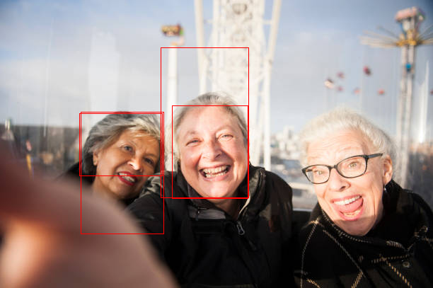
调整区域后

调整区域前
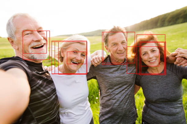
调整区域后

精度和 RCNN 差不多,甚至有些降低了 (为了支持 4G 显存缩放图片了)。不过识别速度有很大的提升,在同一个环境下,Fast-RCNN 处理单张图片只需要 0.4~0.5 秒,而 RCNN 则需要 2 秒左右。


 5905
5905

 被折叠的 条评论
为什么被折叠?
被折叠的 条评论
为什么被折叠?
 到【灌水乐园】发言


