R聚类瞎写

样本点之间的距离 首先利用欧氏距离计算距离矩阵

d<-c(1,2,5,7,9,10)
### 样本点之间的距离
### 首先利用欧氏距离计算距离矩阵
d.mat <- dist(d, method='euclidean',diag=TRUE, upper=F)

> d.mat
  1 2 3 4 5 6
1 0          
2 1 0        
3 4 3 0      
4 6 5 2 0    
5 8 7 4 2 0  
6 9 8 5 3 1 0

R 中用 dist(data, method=) 函数计算观测间的距离。在 dist() 函数中， diag选项决定显示距离阵时是否显示对角线元素， upper 决定显示距离阵时是否显示上三角元素， method 是距离种类 :
• euclidean 欧式距离 ;
• manhattan 曼哈顿距离 ;
• maximum 最大（上确界）距离 ;
• minkowski 闵可夫斯基距离 ;
• canberra 兰氏距离。
本例的 6 个评分取值范围相近，所以不需要标准化。如果变量取值范围差别很大，
在计算距离前一般应该把每列标准化 (scale() 函数 )

用最短距离法聚类

> res1 <- hclust(d.mat, method='single'); res1

Call:
hclust(d = d.mat, method = "single")

Cluster method   : single 
Distance         : euclidean 
Number of objects: 6 

hclust() 函数中选项 method 选择系统聚类的类间距离，包括：
• single 最短距离法，
• complete 最大距离法
• average 类平均法
• median 中间距离法
• centrold 重心法
• ward Ward 法

对 hclust() 的输出结果用 plot() 画聚类树状图：

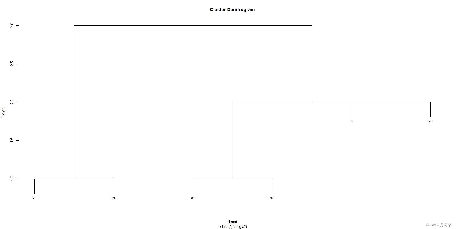
观测的左右关系不代表距离，两类相连时纵轴的高度才代表两类之间的距离，距离越大，越不应该合并到一起。
对 hclust() 的输出结果用 cutree(tree, k=) 得到每个观测的分类号，输出类号组成的向量。注意聚类方法的结果是一些分类，具体的类编号并没有意义。

> cut1 <- cutree(res1, k=2); cut1
[1] 1 1 2 2 2 2

结果 cut1 是分为两类后每个观测的类编号。
用并列盒形图验证分类：

> boxplot(t(as.matrix(d)))

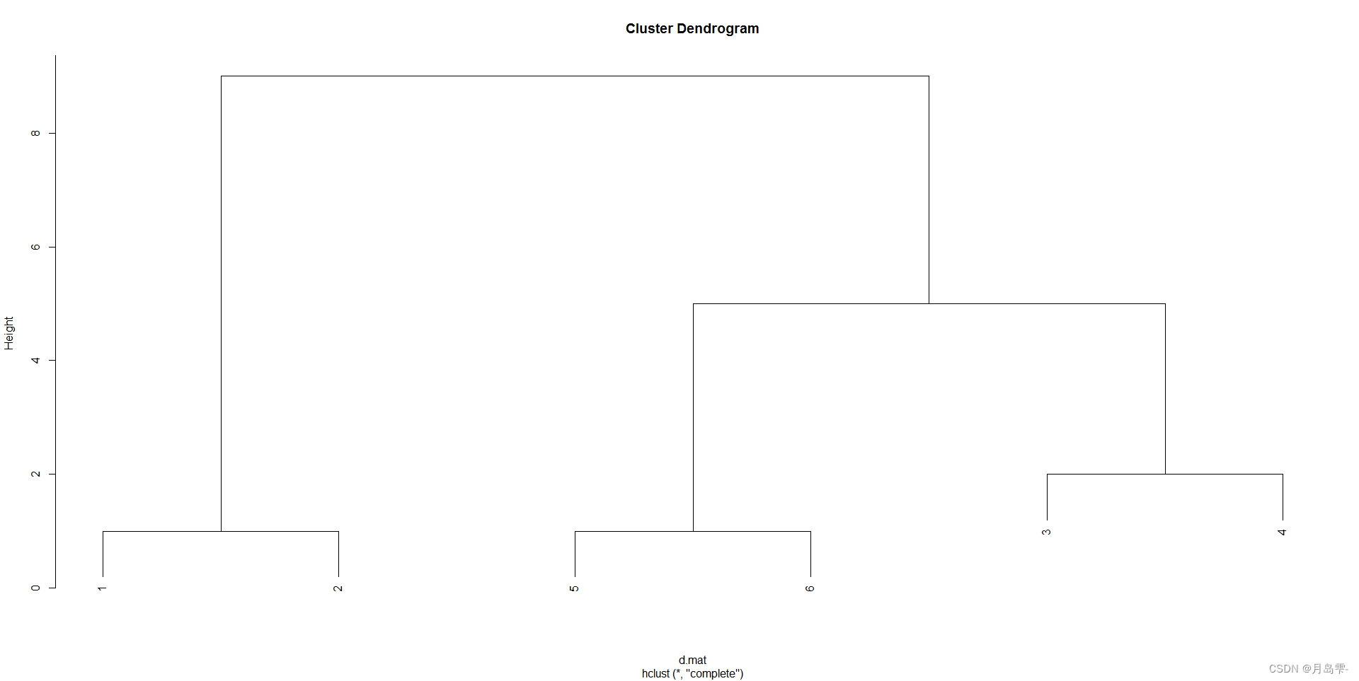
用最长距离法聚类

> res2 <- hclust(d.mat, method='complete'); res2

Call:
hclust(d = d.mat, method = "complete")

Cluster method   : complete 
Distance         : euclidean 
Number of objects: 6 

plot(res2)

> cut2 <- cutree(res2, k=2); cut2
[1] 1 1 2 2 2 2

> cut2b <- cutree(res2, k=3); cut2b
[1] 1 1 2 2 3 3