


 本文围绕Transformer模型展开,介绍其可减少顺序计算,处理长序列更优。详细阐述模型体系结构,包括编码器和解码器堆栈、注意力机制(缩放点产品注意力、多头注意力等)、位置级前馈网络、嵌入和softmax以及位置编码等内容,还给出代码和论文地址。
目录
一.注意
- 以下翻译均来自百度翻译,如有翻译不精准的地方,请谅解!
- 本篇文章是通过对论文的阅读和视频讲解以及笔者自己的一些思路,如有错误请指正,并时刻交流!
- 代码官方地址:https://github.com/huggingface/transformers
- 论文下载地址:https://paperswithcode.com/paper/attention-is-all-you-need
- B站老师讲解视频地址:https://www.bilibili.com/video/BV1pu411o7BE/?spm_id_from=333.999.0.0
二.引言
三.相关工作
原文:The goal of reducing sequential computation also forms the foundation of the Extended Neural GPU,ByteNet and ConvS2S , all of which use convolutional neural networks as basic building block, computing hidden representations in parallel for all input and output positions. In these models, the number of operations required to relate signals from two arbitrary input or output positions grows in the distance between positions, linearly for ConvS2S and logarithmically for ByteNet. This makes it more difficult to learn dependencies between distant positions . In the Transformer this is reduced to a constant number of operations, albeit at the cost of reduced effective resolution due to averaging attention-weighted positions, an effect we counteract with Multi-Head Attention as described in section 3.2.
翻译:减少顺序计算的目标也构成了扩展神经GPU、ByteNet和ConvS2S的基础,所有这些都使用卷积神经网络作为基本构建块,并行计算所有输入和输出位置的隐藏表示。在这些模型中,关联来自两个任意输入或输出位置的信号所需的操作数量随着位置之间的距离而增加,对ConvS2S是线性的,对于ByteNet是对数的。这使得学习远距离位置之间的依赖关系变得更加困难。在Transformer中,这被减少到恒定数量的操作,尽管代价是由于平均注意力加权位置而降低了有效分辨率,如第3.2节所述,我们用多头注意力来抵消这种影响。
解读:在卷积神经网络中,卷积在面对长序列时,会产生累积的效果,当累计到一定程度才能到达序列的结尾,此外,卷积还具有多通道输出的效果。因此,transformer的注意力机制在处理长序列时,可以每一次看到所有并学习卷积的多通道输出(多头注意力).
entirely on self-attention to compute representations of its input and output without using sequence aligned RNNs or convolution. In the following sections, we will describe the Transformer, motivate self-attention and discuss its advantages over models such as and.
四.模型体系结构
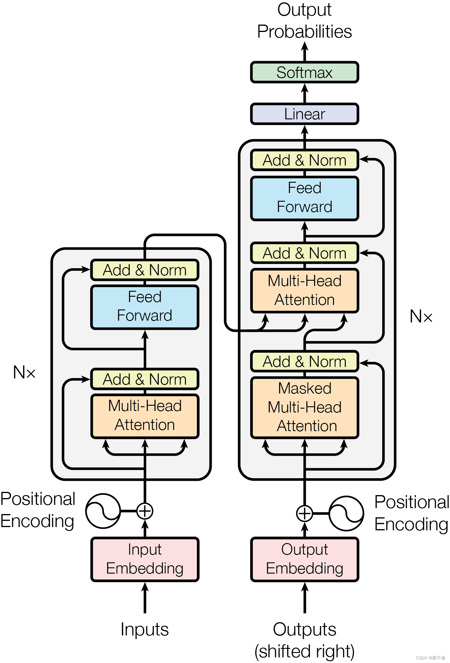
原文:Most competitive neural sequence transduction models have an encoder-decoder structure .Here, the encoder maps an input sequence of symbol representations (x1, ..., xn) to a sequence of continuous representations z = (z1, ..., zn). Given z, the decoder then generates an output sequence (y1, ..., ym) of symbols one element at a time. At each step the model is auto regressive, consuming the previously generated symbols as additional input when generating the next. The Transformer follows this overall architecture using stacked self-attention and point-wise, fully connected layers for both the encoder and decoder, shown in the left and right halves of Figure 1, respectively.
翻译:大多数竞争性神经序列转导模型都具有编码器-解码器结构。这里,编码器将符号表示的输入序列(x1,…,xn)映射到连续表示的序列z=(z1,…,zn)。给定z,解码器然后一次一个元素地生成符号的输出序列(y1,…,ym)。在每一步,模型都是自回归的,在生成下一步时,将先前生成的符号作为额外输入。Transformer遵循这一总体架构,使用堆叠的自关注和逐点、完全连接的编码器和解码器层,分别如图1的左半部分和右半部分所示。
1.编码器和解码器堆栈
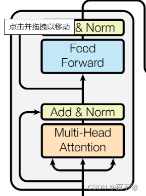
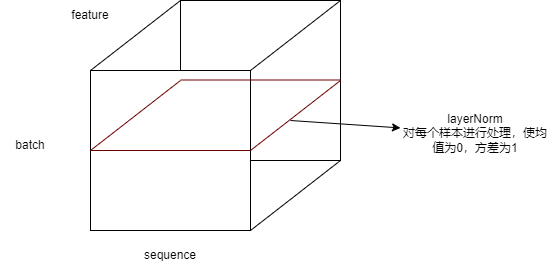
原文:Encoder: The encoder is composed of a stack of N = 6 identical layers. Each layer has two sub-layers. The first is a multi-head self-attention mechanism, and the second is a simple, position-wise fully connected feed-forward network. We employ a residual connection [10] around each of the two sub-layers, followed by layer normalization. That is, the output of each sub-layer is LayerNorm(x + Sublayer(x)), where Sublayer(x) is the function implemented by the sub-layer itself. To facilitate these residual connections, all sub-layers in the model, as well as the embedding layers, produce outputs of dimension dmodel = 512.
翻译:编码器:编码器由N=6个相同层的堆栈组成。每层有两个子层。第一种是多头自注意机制,第二种是简单的位置全连接前馈网络。我们在两个子层中的每一个子层周围使用残差连接[10],然后进行层归一化。也就是说,每个子层的输出是LayerNorm(x+Sublayer(x)),其中Sublayer(x)是由子层本身实现的函数。为了促进这些残余连接,模型中的所有子层以及嵌入层产生维度dmodel=512的输出。
解读:左侧的编码器,如图所示,这个是一个层,在编码器中有六个这种结构。那么在这种结构中也叫层,每层中都存在两个子层,分别为多头自注意力机制和位置全连接前馈网络(mlp)。
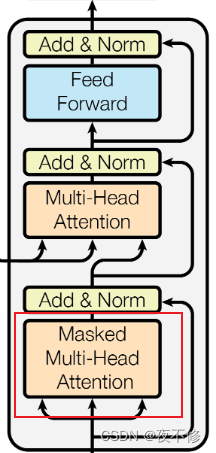
原文:Decoder: The decoder is also composed of a stack of N = 6 identical layers. In addition to the two sub-layers in each encoder layer, the decoder inserts a third sub-layer, which performs multi-head attention over the output of the encoder stack. Similar to the encoder, we employ residual connections around each of the sub-layers, followed by layer normalization. We also modify the self-attention sub-layer in the decoder stack to prevent positions from attending to subsequent positions. This masking, combined with fact that the output embeddings are offset by one position, ensures that the predictions for position i can depend only on the known outputs at positions less than.
翻译:解码器:解码器也是由N=6个相同层的堆栈组成的。除了每个编码器层中的两个子层之外,解码器还插入第三个子层,该第三子层对编码器堆栈的输出执行多头关注。与编码器类似,我们在每个子层周围使用残差连接,然后进行层归一化。我们还修改了解码器堆栈中的自注意子层,以防止位置关注后续位置。这种掩蔽,再加上输出嵌入偏移一个位置的事实,确保了对位置i的预测只能取决于小于的位置处的已知输出。
解读:在下面的解码器中,我们要注意红色框中的内容,它实现了在t时间的时候不会看到t时间之后的输入,以保证训练和预测的时候行为一致。
2.注意力
原文: An attention function can be described as mapping a query and a set of key-value pairs to an output, where the query, keys, values, and output are all vectors. The output is computed as a weighted sum of the values, where the weight assigned to each value is computed by a compatibility function of the query with the corresponding key.
翻译:注意力函数可以描述为将查询和一组键值对映射到输出,其中查询、键、值和输出都是向量。输出被计算为值的加权和,其中分配给每个值的权重由查询与相应关键字的兼容性函数计算。
2.1缩放点产品注意力
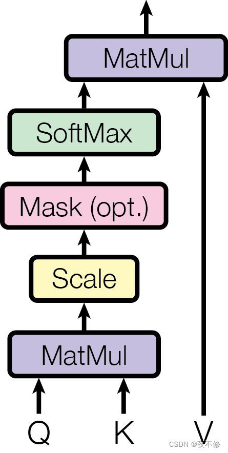
原文:We call our particular attention "Scaled Dot-Product Attention" (Figure 2). The input consists of queries and keys of dimension dk, and values of dimension dv. We compute the dot products of the Figure 2: (left) Scaled Dot-Product Attention. (right) Multi-Head Attention consists of several attention layers running in parallel. query with all keys, divide each by √ dk, and apply a softmax function to obtain the weights on the values. In practice, we compute the attention function on a set of queries simultaneously, packed together into a matrix Q. The keys and values are also packed together into matrices K and V . We compute the matrix of outputs as:
翻译:我们将我们的特别关注称为“标度点产品关注”(图2)。输入包括维度dk的查询和键以及维度dv的值。我们计算图2的点积:(左)缩放点积注意力。(右)多头注意力由几个平行运行的注意力层组成。使用所有键进行查询,将每个键除以√dk,然后应用softmax函数来获得值的权重。在实践中,我们同时计算一组查询的注意力函数,并将其打包成矩阵Q。键和值也打包成矩阵K和V。我们将输出矩阵计算为:
两个最常用的注意力函数是加性注意力和点积(乘法)注意力。点积注意力与我们的算法相同,只是比例因子为。加性注意力使用具有单个隐藏层的前馈网络来计算兼容性函数。虽然两者在理论复杂性上相似,但点积注意力在实践中要快得多,空间效率更高,因为它可以使用高度优化的矩阵乘法代码来实现。虽然对于较小的dk值,这两种机制的表现相似,但在不缩放较大的dk的情况下,相加注意力优于点积注意力。我们怀疑,对于较大的dk值,点积的大小会变大,从而将softmax函数推向具有极小梯度的区域。为了抵消这种影响,我们按比例缩放点积.
解读:在下图中,由于attention在处理ht时,可以获取到ht之前的内容和之后的内容,那么为了防止ht之后的内容对结果的影响,通过下方的mask使ht之后的权重很小,在经过softmax后就会等于0.
2.2多头注意力
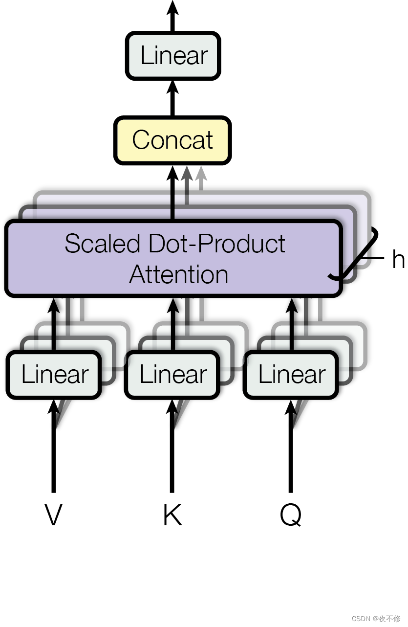
原文:Instead of performing a single attention function with dmodel-dimensional keys, values and queries,we found it beneficial to linearly project the queries, keys and values h times with different, learned linear projections to dk, dk and dv dimensions, respectively. On each of these projected versions of queries, keys and values we then perform the attention function in parallel, yielding dv-dimensional output values. These are concatenated and once again projected, resulting in the final values, as depicted in Figure 2.Multi-head attention allows the model to jointly attend to information from different representation subspaces at different positions. With a single attention head, averaging inhibits this.
其中投影是参数矩阵Wi-Q∈Rdmodel×dk,Wi-K∈R dmodel x dk,Wi-Fi∈R dm odel×dv和WO∈R hdv×dmodel。在这项工作中,我们使用了h=8个平行的注意力层或头部。对于其中的每一个,我们使用dk=dv=dmodel/h=64。由于每个头部的维数降低,总计算成本与全维度的单头注意力相似。
2.3注意点在我们的模型中的应用
原文:The Transformer uses multi-head attention in three different ways:
-
In "encoder-decoder attention" layers, the queries come from the previous decoder layer,and the memory keys and values come from the output of the encoder. This allows everyposition in the decoder to attend over all positions in the input sequence. This mimics thetypical encoder-decoder attention mechanisms in sequence-to-sequence models such as
-
The encoder contains self-attention layers. In a self-attention layer all of the keys, valuesand queries come from the same place, in this case, the output of the previous layer in theencoder. Each position in the encoder can attend to all positions in the previous layer of theencoder.
-
Similarly, self-attention layers in the decoder allow each position in the decoder to attend toall positions in the decoder up to and including that position. We need to prevent leftwardinformation flow in the decoder to preserve the auto-regressive property. We implement thisinside of scaled dot-product attention by masking out (setting to −∞) all values in the inputof the softmax which correspond to illegal connections. See Figure 2.
翻译: Transformer以三种不同的方式使用多头注意力:
-
在“编码器-解码器注意力”层中,查询来自前一个解码器层,并且存储器密钥和值来自编码器的输出。这允许解码器中的位置,以关注输入序列中的所有位置。这模仿了序列到序列模型中的典型编码器-解码器注意力机制,例如
-
编码器包含自关注层。在自我关注层中,所有的键、值和查询来自同一个位置,在这种情况下,是中上一层的输出编码器。编码器中的每个位置都可以处理的前一层中的所有位置编码器。
-
类似地,解码器中的自关注层允许解码器中的每个位置关注解码器中直到并包括该位置的所有位置。我们需要防止向左解码器中的信息流以保持自回归特性。我们实施这一点通过屏蔽(设置为-∞)输入中的所有值来引起缩放点积内部的注意对应于非法连接的softmax的。见图2。
解读: 在下方的编码器结构中,我们的输入复制成为了三份,分别作为key,value,query,本质上输出就是与输入的不同相似度。解码器输入也是,masked前面也提到过,不让他看到后面的东西。但解码器中的Muti-Head Attention,输入的key和value来自编码器,query来自解码器,
3.位置级的前馈网络
原文:In addition to attention sub-layers, each of the layers in our encoder and decoder contains a fully connected feed-forward network, which is applied to each position separately and identically. This consists of two linear transformations with a ReLU activation in between
翻译:除了注意力子层之外,我们的编码器和解码器中的每个层都包含一个完全连接的前馈网络,该网络分别且相同地应用于每个位置。这包括两个线性变换,其间有ReLU激活
虽然线性变换在不同的位置上是相同的,但它们在不同的层之间使用不同的参数。另一种描述方式是将其描述为核大小为1的两个卷积。输入和输出的维度为dmodel=512,内层的维度dff=2048。
4.嵌入和softmax
原文:Similarly to other sequence transduction models, we use learned embeddings to convert the input tokens and output tokens to vectors of dimension dmodel. We also use the usual learned linear transformation and softmax function to convert the decoder output to predicted next-token probabilities. In our model, we share the same weight matrix between the two embedding layers and the pre-softmax linear transformation, similar to. In the embedding layers, we multiply those weights by √ dmodel.
翻译:与其他序列转导模型类似,我们使用学习嵌入将输入令牌和输出令牌转换为维度dmodel的向量。我们还使用通常学习的线性变换和softmax函数将解码器输出转换为预测的下一个令牌概率。在我们的模型中,我们在两个嵌入层和预softmax线性变换之间共享相同的权重矩阵,类似于。在嵌入层中,我们将这些权重乘以√dmodel。
5.位置编码
原文:Since our model contains no recurrence and no convolution, in order for the model to make use of the order of the sequence, we must inject some information about the relative or absolute position of the tokens in the sequence. To this end, we add "positional encodings" to the input embeddings at the Table 1: Maximum path lengths, per-layer complexity and minimum number of sequential operations for different layer types. n is the sequence length, d is the representation dimension, k is the kernel size of convolutions and r the size of the neighborhood in restricted self-attention.bottoms of the encoder and decoder stacks. The positional encodings have the same dimension dmodel as the embeddings, so that the two can be summed. There are many choices of positional encodings, learned and fixed. In this work, we use sine and cosine functions of different frequencies:
where pos is the position and i is the dimension. That is, each dimension of the positional encoding corresponds to a sinusoid. The wavelengths form a geometric progression from 2π to 10000 · 2π. We chose this function because we hypothesized it would allow the model to easily learn to attend by relative positions, since for any fixed offset k, P Epos+k can be represented as a linear function of P Epos. We also experimented with using learned positional embeddings [8] instead, and found that the two versions produced nearly identical results (see Table 3 row (E)). We chose the sinusoidal version because it may allow the model to extrapolate to sequence lengths longer than the ones encountered during training.

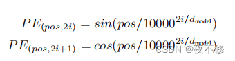
翻译:由于我们的模型不包含递归和卷积,为了让模型利用序列的顺序,我们必须注入一些关于令牌在序列中的相对或绝对位置的信息。为此,我们在表1的输入嵌入中添加了“位置编码”:不同层类型的最大路径长度、每层复杂性和最小顺序操作数。n是序列长度,d是表示维数,k是卷积的核大小,r是编码器和解码器堆栈的限制自关注基底中的邻域的大小。位置编码与嵌入具有相同的维度dmodel,因此可以将两者相加。有许多位置编码的选择,有学习的和固定的。在这项工作中,我们使用不同频率的正弦和余弦函数:
其中pos是位置,i是尺寸。也就是说,位置编码的每个维度对应于正弦曲线。波长形成从2π到10000·2π的几何级数。我们选择这个函数是因为我们假设它可以让模型很容易地学会通过相对位置来关注,因为对于任何固定的偏移k,P Epos+k可以表示为P Epos的线性函数。我们还使用学习的位置嵌入[8]进行了实验,发现这两个版本产生了几乎相同的结果(见表3第(E)行)。我们选择正弦版本是因为它可以允许模型外推到比训练期间遇到的序列长度更长的序列长度。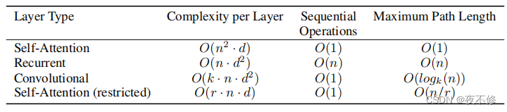


 被折叠的 条评论
为什么被折叠?
被折叠的 条评论
为什么被折叠?
 到【灌水乐园】发言


