


这个项目是在ANN之后的一个项目,有了BP神经网络的基础,RNN和LSTM能够更好的理解。虽然仍然不是特别深入的学习,但是可以有了初步的应用了。
不同于全连接的深度神经网络(Deep Neural Networks, DNN)和卷积神经网络(Convolutional Neural Network, CNN),每层神经元只能向上传播,样本处理各个时刻相互独立,因而无法对时间序列上的变化建模,循环神经网络(recurrent neural network, RNN)可以进行时间序列建模。而基于长短期记忆单元(Long Short-term memory, LSTM)的RNN模型可以缓解长序列训练过程中梯度消失和梯度爆炸问题。(张军阳)
本项目采取基于Tensorflow2搭建优化神经网络的方法,使用循环神经网络(RNN)以及长短期记忆递归神经网络(LSTM)对收集到的外汇数据进行数据分析。使用的神经网络预测方法,其原理是模拟人脑的抽象描述功能从而对事件序列的远期走势进行预测分析的。而采取的循环网络RNN这种研究方法在对序列化数据的处理中是非常高效的深度学习模型。长短期记忆网络LSTM也是一种时间循环神经网络,它是为了解决一般的RNN存在的账期以来问题而专门设计出来的,因此,本项目主要使用RNN进行外汇价格预测分析,辅以LSTM来进行改进。本项目可以观察simpleRNN和LSTM改进后RNN的区别。
SimpleRNN
1.数据引入
os.environ['TF_CPP_MIN_LOG_LEVEL'] = '2'

usdcnh = pd.read_csv('USDCNH.csv')                                #读取汇率文件

traning_set = usdcnh.iloc[1:3601 , 1:2].values                          #将前3600行数据作为训练集,取[1,2)列,即第二列,‘open’列数据
test_set = usdcnh.iloc[3601:4801 , 1:2].values                          #将第3600至4800行数据作为测试集
2.训练集与测试集处理
#归一化
sc = MinMaxScaler(feature_range=(0,1))
training_set_scaled = sc.fit_transform(traning_set)             #归一化训练集数据
test_set_scaled = sc.fit_transform(test_set)                    #归一化测试集数据

x_train = []    #存储训练集输入特征
y_train = []    #存储训练集标签

x_test = []     #存储测试集输入特征
y_test = []     #存储测试集标签

for i in range(60,len(training_set_scaled)):                    #遍历训练集数据
    x_train.append(training_set_scaled[i-60:i,0])               #每“连续”60天([i-60,i))数据作为一个输入特征
    y_train.append(training_set_scaled[i,0])                    #将第61天(i)数据作为标签

np.random.seed(17)
np.random.shuffle(x_train)                                      #使用指定种子来打乱数据(目的是使测试时结果相对一致)
np.random.seed(17)
np.random.shuffle(y_train)
tf.random.set_seed(17)                                          #设定全图随机种子
x_train,y_train = np.array(x_train),np.array(y_train)           #将list格式转变为nparray格式、
3.模型构建
将x_train转变为RNN指定的输入格式:
[输入样本数(使用nparray的shape属性中行属性标识),循环核时间展开步数,每个时间步输入特征个数]
这时将选定的3600行数据输入,即3600分钟的开盘价,循环核时间展开步数为60,即输入60分钟的''open'价格,预测第61分钟的'open'价格
每个时间送入的是每个分钟的'open'价格,只有一个数据,因此每个时间步输入特征个数为1
x_train = np.reshape(x_train,(x_train.shape[0],60,1))

for i in range(60,len(test_set_scaled)):                        #遍历测试集数据
    x_test.append(test_set_scaled[i-60:i,0])                    #与训练集类似,将“连续”60天([i-60,i))数据作为一个输入特征
    y_test.append(test_set_scaled[i,0])                         #与训练集类似,将第61天(i)数据作为对应的标签

x_test,y_test = np.array(x_test) , np.array(y_test)
x_test = np.reshape(x_test,(x_test.shape[0],60,1))              #与训练集类似,转变为nparray格式,转变为RNN指定的输入格式

model = models.Sequential([                                     #用Sequential搭建神经网络
    SimpleRNN(200,return_sequences = True),                     #第一层循环计算层记忆体设定为200个,每个时间步推送ht给下一层,默认激活函数‘tanh’
    Dropout(0.2),                                               #dropout比率设定为0.2
    SimpleRNN(300),                                             #第二层记忆体设定为300个
    Dropout(0.2),
    Dense(1)                                                    #由于输出的是第61分钟的‘open’价格,一个数,所以dense设定为1
    ])

model.compile(optimizer = optimizers.Adam(0.001),               #配置训练方法,使用Adam优化器
              loss = 'mse')                                     #使用均方误差损失函数.该应用不观测准确率,只观测loss,因此删去metrics选项
4.断点续训
#设置断点续训
checkpoint_save_path = 'checkpoint/forchange.ckpt'
if os.path.exists(checkpoint_save_path + '.index'):
    print('=====================load the model=====================')
    model.load_weights(checkpoint_save_path)
cp_callback = callbacks.ModelCheckpoint(filepath = checkpoint_save_path,
                                        save_weigths_only = True,           #仅保存模型的权重,而不保存完整模型
                                        save_best_only = True,              #被监测数据的最佳模型不会被覆盖
                                        monitor = 'val_loss')               #需要监测的评估指标为‘val_loss’(测试集整体损失值)
5.执行训练
fit函数执行训练过程!
输入为x_train,输出为y_train,每一个batch大小即训练一次网络所用的样本数为64,
全部样本被迭代50次后停止,即epochs为50;
指定验证数据为测试集(x_test,y_test),验证数据的epoch为1;
当监视的变量停止改善时,停止训练,防止模型过拟合。
#history中包含训练集loss,测试集loss:val_loss,训练集准确率sprase_categorical_accuracy,测试集准确率val_sprase_categorical_accuracy
history = model.fit(x_train,y_train,batch_size = 64,epochs= 50,
                    validation_data=(x_test,y_test),
                    validation_freq = 1,
                    callbacks = [cp_callback])
6.打印出网络结构和参数统计
model.summary()
#参数提取
file = open('weights.txt','w') #参数提取
for v in model.trainable_variables:
file.write(str(v.name)+'\n')
file.write(str(v.shape)+'\n')
file.write(str(v.numpy())+'\n')
file.close()
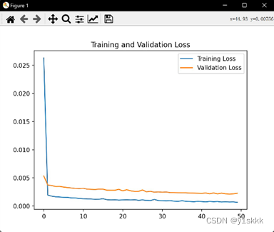
loss = history.history['loss'] #提取训练集loss
val_loss = history.history['val_loss'] #提取测试集loss
#可视化
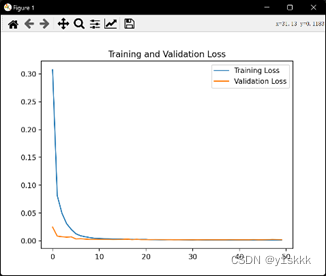
plt.plot(loss,label = 'Training Loss') #绘出训练集loss和测试集loss图像
plt.plot(val_loss,label = 'Validation Loss')
plt.title('Training and Validation Loss')
plt.legend()
plt.show()
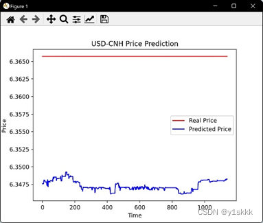
predict_forex_price = model.predict(x_test) #测试集输入模型进行预测
predict_forex_price = sc.inverse_transform(predict_forex_price) #反归一化预测值
real_forex_price = sc.inverse_transform(test_set[60:]) #反归一化真实值
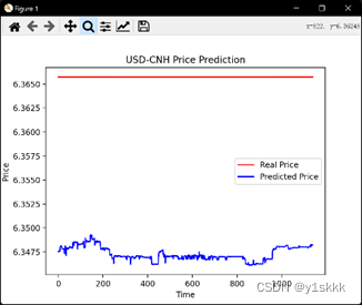
plt.plot(real_forex_price,color = 'red',label = 'Real Price') #绘出测试集真实值和预测值图像
plt.plot(predict_forex_price,color = 'blue',label = 'Predicted Price')
plt.title('USD-CNH Price Prediction')
plt.xlabel('Time')
plt.ylabel('Price')
plt.legend()
plt.show()
#模型评价
mse = mean_squared_error(predict_forex_price,real_forex_price) #均方误差
rmse = math.sqrt(mean_squared_error(predict_forex_price,real_forex_price)) #均方根误差
mae = mean_absolute_error(predict_forex_price,real_forex_price) #平均绝对误差
print('均方误差:%.6f'%mse)
print('均方根误差:%.6f'%rmse)
print('平均绝对误差:%.6f'%mae)7.结果分析
我们采用了大小样本来对比结果,小样本为训练集3600个,测试集1200个;大样本为训练集36000个,测试集12000个,发现普通RNN模型存在着严重的梯度消失问题。
|
小样本的误差结果如下:
均方误差:0.000031
均方根误差:0.005601
平均绝对误差:0.005601;
大样本的误差结果如下:
均方误差:0.039165
均方根误差:0.197901
平均绝对误差:0.197799
LSTM
1.数据引入
os.environ['TF_CPP_MIN_LOG_LEVEL'] = '2'

usdcnh = pd.read_csv('USDCNH.csv')                                #读取汇率文件

traning_set = usdcnh.iloc[1:36001 , 1:2].values                     #将前3600行数据作为训练集,取[1,2)列,即第二列,‘open’列数据
test_set = usdcnh.iloc[36001:48001 , 1:2].values                    #将第3600至4800行数据作为测试集
2.训练集与测试集数据处理
#归一化
sc = MinMaxScaler(feature_range=(0,1))
training_set_scaled = sc.fit_transform(traning_set)             #归一化训练集数据
test_set_scaled = sc.fit_transform(test_set)                    #归一化测试集数据

x_train = []    #存储训练集输入特征
y_train = []    #存储训练集标签

x_test = []     #存储测试集输入特征
y_test = []     #存储测试集标签

for i in range(60,len(training_set_scaled)):                    #遍历训练集数据
    x_train.append(training_set_scaled[i-60:i,0])               #每“连续”60天([i-60,i))数据作为一个输入特征
    y_train.append(training_set_scaled[i,0])                    #将第61天(i)数据作为标签

np.random.seed(17)
np.random.shuffle(x_train)                                      #使用指定种子来打乱数据(目的是使测试时结果相对一致)
np.random.seed(17)
np.random.shuffle(y_train)
tf.random.set_seed(17)                                          #设定全图随机种子
x_train,y_train = np.array(x_train),np.array(y_train)           #将list格式转变为nparray格式、
3.构建模型
将x_train转变为RNN指定的输入格式:
[输入样本数(使用nparray的shape属性中行属性标识),循环核时间展开步数,每个时间步输入特征个数]
这时将选定的3600行数据输入,即3600分钟的开盘价,循环核时间展开步数为60,即输入60分钟的''open'价格,预测第61分钟的'open'价格
每个时间送入的是每个分钟的'open'价格,只有一个数据,因此每个时间步输入特征个数为1
x_train = np.reshape(x_train,(x_train.shape[0],60,1))

for i in range(60,len(test_set_scaled)):                        #遍历测试集数据
    x_test.append(test_set_scaled[i-60:i,0])                    #与训练集类似,将“连续”60天([i-60,i))数据作为一个输入特征
    y_test.append(test_set_scaled[i,0])                         #与训练集类似,将第61天(i)数据作为对应的标签

x_test,y_test = np.array(x_test) , np.array(y_test)
x_test = np.reshape(x_test,(x_test.shape[0],60,1))              #与训练集类似,转变为nparray格式,转变为RNN指定的输入格式

model = models.Sequential([                                     #用Sequential搭建神经网络
    LSTM(200,return_sequences = True),                     #第一层循环计算层记忆体设定为200个,每个时间步推送ht给下一层,默认激活函数‘tanh’
    Dropout(0.1),                                               #dropout比率设定为0.2
    LSTM(300),                                             #第二层记忆体设定为300个
    Dropout(0.1),
    Dense(1)                                                    #由于输出的是第61分钟的‘open’价格,一个数,所以dense设定为1
    ])

model.compile(optimizer = optimizers.Adam(0.001),               #配置训练方法,使用Adam优化器
              loss = 'mse')                                     #使用均方误差损失函数.该应用不观测准确率,只观测loss,因此删去metrics选项
4.断点续训
checkpoint_save_path = 'checkpoint/forchange.ckpt'
if os.path.exists(checkpoint_save_path + '.index'):
    print('=====================load the model=====================')
    model.load_weights(checkpoint_save_path)
cp_callback = callbacks.ModelCheckpoint(filepath = checkpoint_save_path,
                                        save_weigths_only = True,           #仅保存模型的权重,而不保存完整模型
                                        save_best_only = True,              #被监测数据的最佳模型不会被覆盖
                                        monitor = 'val_loss')               #需要监测的评估指标为‘val_loss’(测试集整体损失值)
5.执行训练
#history中包含训练集loss,测试集loss:val_loss,训练集准确率sprase_categorical_accuracy,测试集准确率val_sprase_categorical_accuracy
history = model.fit(x_train,y_train,batch_size = 64,epochs= 50,
                    validation_data=(x_test,y_test),
                    validation_freq = 1,
                    callbacks = [cp_callback])
6.打印出网络结构和参数统计
model.summary()
#参数提取
file = open('weights.txt','w') #参数提取
for v in model.trainable_variables:
file.write(str(v.name)+'\n')
file.write(str(v.shape)+'\n')
file.write(str(v.numpy())+'\n')
file.close()
loss = history.history['loss'] #提取训练集loss
val_loss = history.history['val_loss'] #提取测试集loss
#可视化
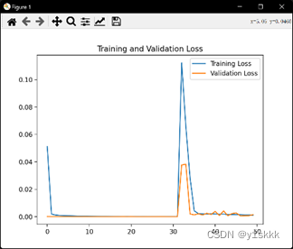
plt.plot(loss,label = 'Training Loss') #绘出训练集loss和测试集loss图像
plt.plot(val_loss,label = 'Validation Loss')
plt.title('Training and Validation Loss')
plt.legend()
plt.show()
predict_forex_price = model.predict(x_test) #测试集输入模型进行预测
predict_forex_price = sc.inverse_transform(predict_forex_price) #反归一化预测值
real_forex_price = sc.inverse_transform(test_set[60:]) #反归一化真实值
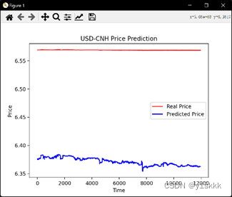
plt.plot(real_forex_price,color = 'red',label = 'Real Price') #绘出测试集真实值和预测值图像
plt.plot(predict_forex_price,color = 'blue',label = 'Predicted Price')
plt.title('USD-CNH Price Prediction')
plt.xlabel('Time')
plt.ylabel('Price')
plt.legend()
plt.show()
#模型评价
mse = mean_squared_error(predict_forex_price,real_forex_price) #均方误差
rmse = math.sqrt(mean_squared_error(predict_forex_price,real_forex_price)) #均方根误差
mae = mean_absolute_error(predict_forex_price,real_forex_price) #平均绝对误差
print('均方误差:%.6f'%mse)
print('均方根误差:%.6f'%rmse)
print('平均绝对误差:%.6f'%mae)7.结果分析
误差数据
样本的误差结果如下:
均方误差:0.000339
均方根误差:0.018416
平均绝对误差:0.018403
由于小样本与大样本在LSTM下结果几乎一致,因此在做该项目时舍弃了:| ; 可以发现,LSTM对RNN的梯度下降是有一定帮助的。
结束语
这是完成的第二个项目,同样是在没有系统性学习的情况下完成的,同样是在参考了很多相关项目的情况下完成的,非常感谢能够有这些资源供参考。突发奇想,这些项目用chatgpt应该可以更快速地完成,更方便地完成了,毕竟这些相关的项目太多了。哈哈:)


 被折叠的 条评论
为什么被折叠?
被折叠的 条评论
为什么被折叠?
 到【灌水乐园】发言


