


 本文介绍了信用评分卡的构建过程,包括数据预处理(如填充缺失值、处理异常值)、数据探索(异常值分析、分布图绘制)和特征工程(WOE和IV值计算)。通过逻辑回归和随机森林模型进行预测,并对模型性能进行了评估。
1.选题背景
信用评分卡是银行等金融机构风险管理一种比较重要的工具,它基于借款人的历史数据和个人信息等数据,通过建立莫种模型来预测借款人的违约概率。这种方法可以帮助金融机构更好地评估风险和决策借款人的信用额度和贷款条件。评分技术采用的是统计模型,是一种很成熟的预测方法,尤其在信用风险评估以及金融风险控制领域更是得到了比较广泛的使用。信用评分卡可以根据客户提供的资料、客户的历史数据、第三方平台(芝麻分、京东、微信等)的数据,对客户的信用进行评估。信用评分卡的建立是以对大量数据的统计分析结果为基础,具有较高的准确性和可靠性。采用的技术主要为数据的处理,逻辑回归分类(对全数值的数据具有很好的分类处理)。主要步骤为:先观察数据,在对数据中的空值,异常值进行处理,处理好后进行相关性分析及woe分析,最后进行分类建立模型,评估模型,得出最后的分数。
2.数据预处理
在这里数据我处理的时候将他乘了四分 没有修改
2.1对数据进行分析
2.1.1 导入相应的库文件
import numpy as np
import pandas as pd
2.1.2 打开相应文件
### 打开文件
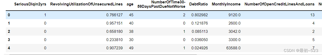
data = pd.read_csv('cs-training.csv')
data = data.iloc[:,1:]
data.head(5)
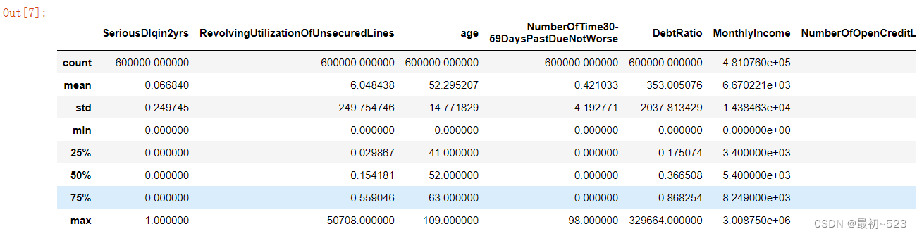
2.1.3各种属性的查看
# 查看特征
data.describe()
## 数据大小
data.shape
(600000, 11)
#空缺值的查看
## 查看空缺值
data.info()
<class 'pandas.core.frame.DataFrame'>
RangeIndex: 600000 entries, 0 to 599999
Data columns (total 11 columns):
 #   Column                                Non-Null Count   Dtype
---  ------                                --------------   -----
 0   SeriousDlqin2yrs                      600000 non-null  int64
 1   RevolvingUtilizationOfUnsecuredLines  600000 non-null  float64
 2   age                                   600000 non-null  int64
 3   NumberOfTime30-59DaysPastDueNotWorse  600000 non-null  int64
 4   DebtRatio                             600000 non-null  float64
 5   MonthlyIncome                         481076 non-null  float64
 6   NumberOfOpenCreditLinesAndLoans       600000 non-null  int64
 7   NumberOfTimes90DaysLate               600000 non-null  int64
 8   NumberRealEstateLoansOrLines          600000 non-null  int64
 9   NumberOfTime60-89DaysPastDueNotWorse  600000 non-null  int64
 10  NumberOfDependents                    584304 non-null  float64
dtypes: float64(4), int64(7)
memory usage: 50.4 MB
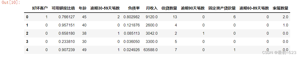
2.2 修改字段
#修改英文字段名为中文字段名
states={
        'SeriousDlqin2yrs':'好坏客户',
        'RevolvingUtilizationOfUnsecuredLines':'可用额度比值',
        'age':'年龄',
        'NumberOfTime30-59DaysPastDueNotWorse':'逾期30-59天笔数',
        'DebtRatio':'负债率',
        'MonthlyIncome':'月收入',
        'NumberOfOpenCreditLinesAndLoans':'信贷数量',
        'NumberOfTimes90DaysLate':'逾期90天笔数',
        'NumberRealEstateLoansOrLines':'固定资产贷款量',
        'NumberOfTime60-89DaysPastDueNotWorse':'逾期60-89天笔数',
        'NumberOfDependents':'家属数量'}
data.rename(columns=states,inplace=True)
data.head()
2.3 处理空值 – 空值通过info查看 月收入和家庭数量的空值较多
# 计算月收入比例
print("月收入缺失比:{:.2%}".format(data['月收入'].isnull().sum()/data.shape[0]))
月收入缺失比:19.82%
# 填充月收入空值通过平均值
data=data.fillna({'月收入':data['月收入'].mean()})
data.info()
<class 'pandas.core.frame.DataFrame'>
RangeIndex: 600000 entries, 0 to 599999
Data columns (total 11 columns):
 #   Column      Non-Null Count   Dtype
---  ------      --------------   -----
 0   好坏客户        600000 non-null  int64
 1   可用额度比值      600000 non-null  float64
 2   年龄          600000 non-null  int64
 3   逾期30-59天笔数  600000 non-null  int64
 4   负债率         600000 non-null  float64
 5   月收入         600000 non-null  float64
 6   信贷数量        600000 non-null  int64
 7   逾期90天笔数     600000 non-null  int64
 8   固定资产贷款量     600000 non-null  int64
 9   逾期60-89天笔数  600000 non-null  int64
 10  家属数量        584304 non-null  float64
dtypes: float64(4), int64(7)
memory usage: 50.4 MB
#  计算家庭数量缺失值的比例
print("家属数量缺失比:{:.2%}".format(data['家属数量'].isnull().sum()/data.shape[0]))
家属数量缺失比:2.62%
# 家庭数量确实率少 可以进行删除处理
data = data.dropna()
data.shape
(584304, 11)
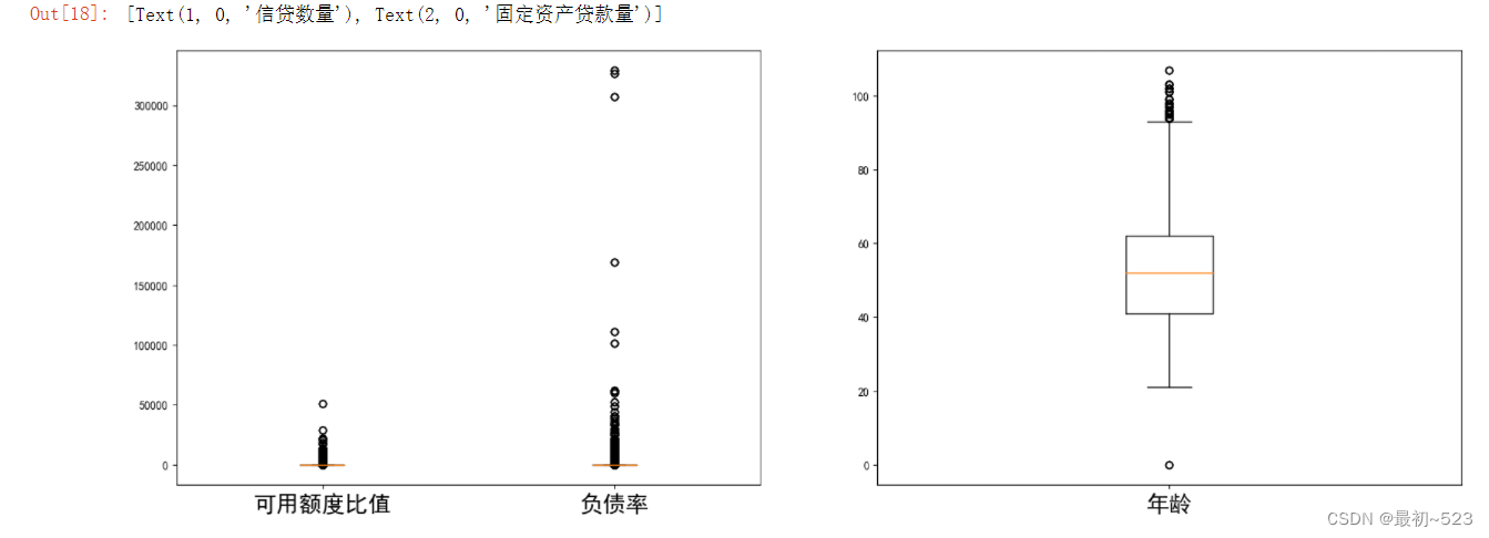
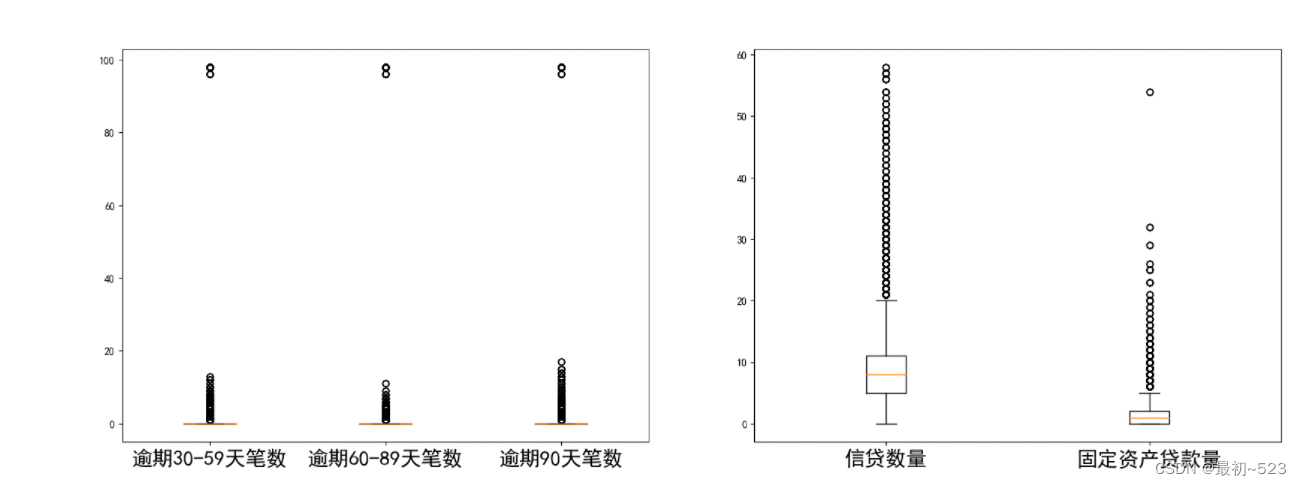
2.4 异常值的处理
2.4.1 异常值的查看
# **2、异常值处理**
# 可以通过箱线图观察异常值```
import matplotlib.pyplot as plt
from pylab import mpl
mpl.rcParams['font.sans-serif'] = ['SimHei']
x1=data['可用额度比值']
x2=data['负债率']
x3=data["年龄"]
x4=data["逾期30-59天笔数"]
x5=data["逾期60-89天笔数"]
x6=data["逾期90天笔数"]
x7=data["信贷数量"]
x8=data["固定资产贷款量"]
fig=plt.figure(figsize=(20,15))
ax1=fig.add_subplot(221)
ax2=fig.add_subplot(222)
ax3=fig.add_subplot(223)
ax4=fig.add_subplot(224)
# ax1.boxplot([x1,x2,x3,x4,x5,x6,x7,x8])
# ax1.set_xticklabels(["可用额度比值","负债率","年龄","逾期30-59天笔数","逾期60-89天笔数","逾期90天笔数","信贷数量","固定资产贷款量"], fontsize=20)
ax1.boxplot([x1,x2])
ax1.set_xticklabels(["可用额度比值","负债率"], fontsize=20)
ax2.boxplot([x3])
ax2.set_xticklabels(["年龄"], fontsize=20)
ax3.boxplot([x4,x5,x6])
ax3.set_xticklabels(["逾期30-59天笔数","逾期60-89天笔数","逾期90天笔数"], fontsize=20)
ax4.boxplot([x7,x8])
ax4.set_xticklabels(["信贷数量","固定资产贷款量"], fontsize=20)
2.4.2 异常值进行处理 消除有问题的数据
data=data[data['可用额度比值']<1]
data=data[data['年龄']>0]
data=data[data['逾期30-59天笔数']<80]
data=data[data['逾期60-89天笔数']<80]
data=data[data['逾期90天笔数']<80]
data=data[data['固定资产贷款量']<50]
data.shape
(570236, 11)
3.数据探索
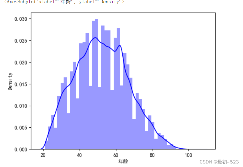
3.1 对单个变量进行探索
3.1.1 对年龄进行探索分析
import seaborn as sns
age = data['年龄']
sns.distplot(age,color='blue')
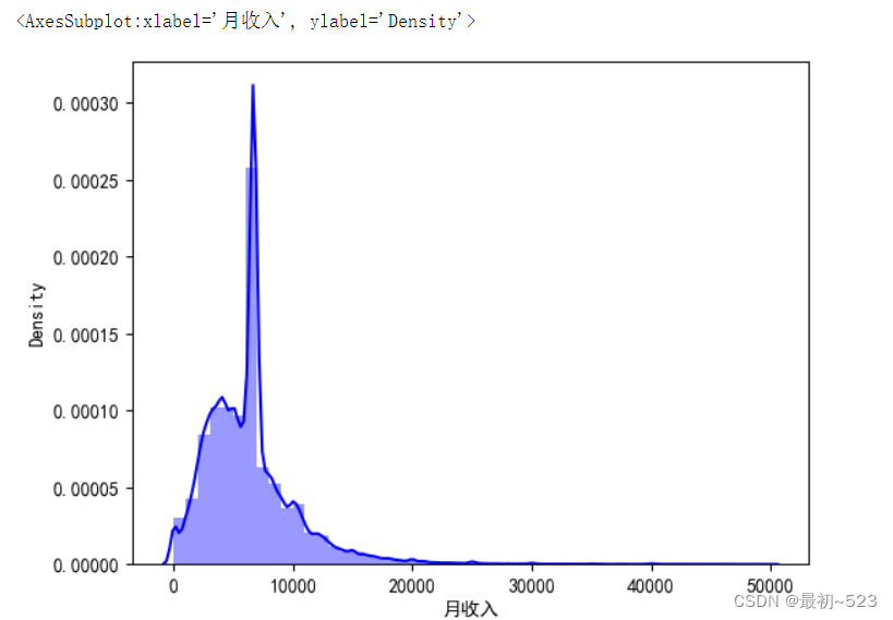
# 对月收入进行探索分析
mi = data[data['月收入']<50000]['月收入']
sns.distplot(mi,color='blue')
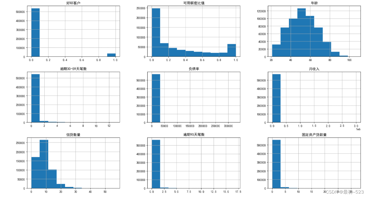
3.2 判断各个特征变量是否满足统计基本假设,即连续型变量应该满足近似正态分布的假设。分别绘制直方图进行分析
data.hist(figsize=(20,15))
array([[<AxesSubplot:title={'center':'好坏客户'}>,
        <AxesSubplot:title={'center':'可用额度比值'}>,
        <AxesSubplot:title={'center':'年龄'}>],
       [<AxesSubplot:title={'center':'逾期30-59天笔数'}>,
        <AxesSubplot:title={'center':'负债率'}>,
        <AxesSubplot:title={'center':'月收入'}>],
       [<AxesSubplot:title={'center':'信贷数量'}>,
        <AxesSubplot:title={'center':'逾期90天笔数'}>,
        <AxesSubplot:title={'center':'固定资产贷款量'}>],
       [<AxesSubplot:title={'center':'逾期60-89天笔数'}>,
        <AxesSubplot:title={'center':'家属数量'}>, <AxesSubplot:>]],
      dtype=object)

3.3 分析年龄于违约客户数的变换关系比给出可视化输出
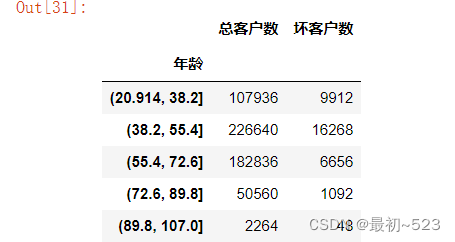
3.3.1 观察数据 中总客户数的情况
age_cut=pd.cut(data['年龄'],5)
age_cut_group=data['好坏客户'].groupby(age_cut).count()
age_cut_group
年龄
(20.914, 38.2]    107936
(38.2, 55.4]      226640
(55.4, 72.6]      182836
(72.6, 89.8]       50560
(89.8, 107.0]       2264
Name: 好坏客户, dtype: int64
3.3.2 观察数据中坏客户剩余情况
age_cut1=pd.cut(data['年龄'],5)
age_cut_group1=data['好坏客户'].groupby(age_cut).sum()
age_cut_group1
年龄
(20.914, 38.2]     9912
(38.2, 55.4]      16268
(55.4, 72.6]       6656
(72.6, 89.8]       1092
(89.8, 107.0]        48
Name: 好坏客户, dtype: int64
3.3.3 将总客户计算出来 并合并成Dataframe 数据形式
goods_cus =pd.merge(pd.DataFrame(age_cut_group),pd.DataFrame(age_cut_group1),left_index=True,right_index=True)
goods_cus.rename(columns={'好坏客户_x':'总客户数','好坏客户_y':'坏客户数'},inplace=True)
goods_cus
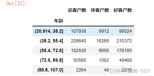
3.3.4 计算出好客户 并插入Dataframe数据中
goods_cus.insert(2,"好客户数",goods_cus["总客户数"]-goods_cus["坏客户数"])
goods_cus
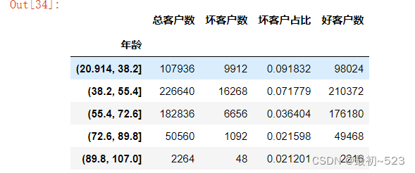
3.3.5 计算坏客户占比 并添加数据
goods_cus.insert(2,"坏客户占比",goods_cus["坏客户数"]/goods_cus["总客户数"])
goods_cus
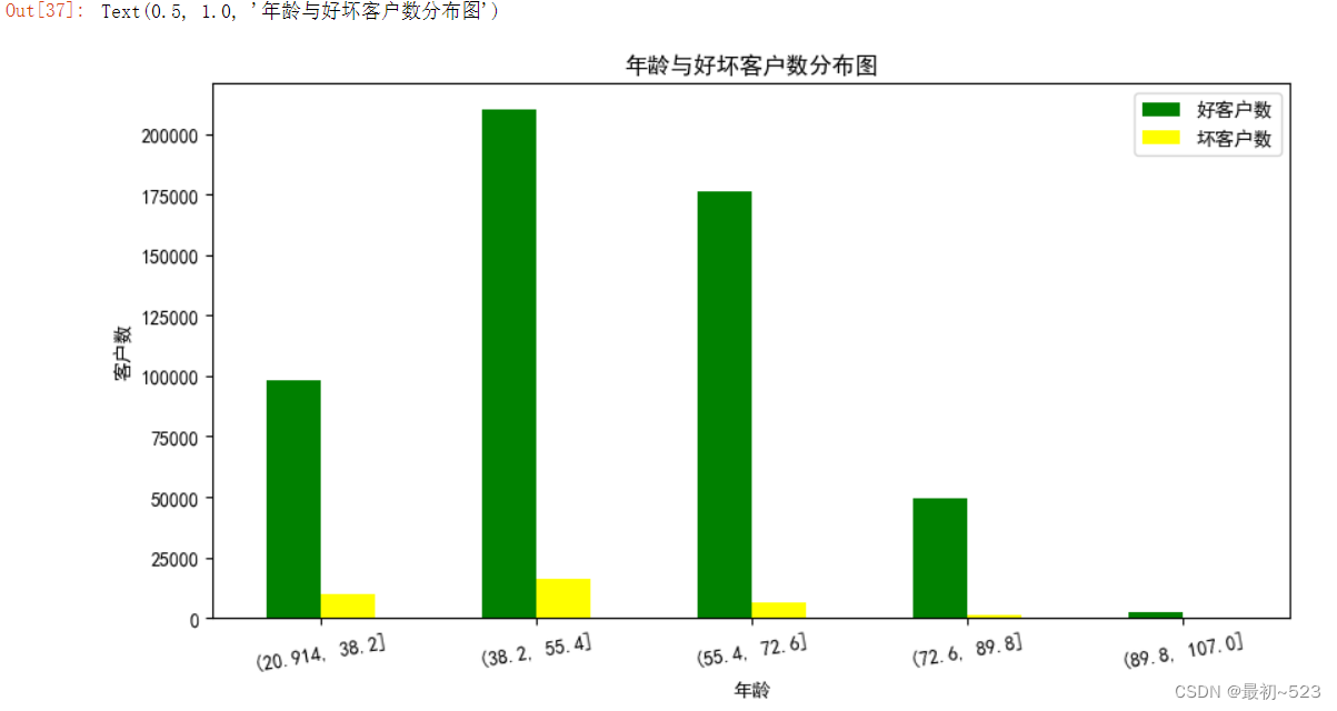
3.3.6 年龄与好坏客户的柱状图
ax1=goods_cus[["好客户数","坏客户数"]].plot.bar(figsize=(10,5 ),color=['green', 'yellow'])
ax1.set_xticklabels(goods_cus.index,rotation=10)
ax1.set_ylabel("客户数")
ax1.set_title("年龄与好坏客户数分布图")
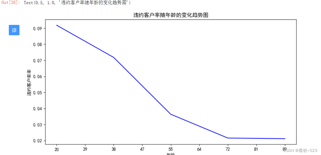
3.3.7 年龄与坏客户的折线图
ax11=goods_cus["坏客户占比"].plot(figsize=(10,5),color=['blue'])
ax11.set_xticklabels([0,20,29,38,47,55,64,72,81,89,98])
ax11.set_ylabel("违约客户率率")
ax11.set_title("违约客户率随年龄的变化趋势图")
4.特征探索
WOE
WOE(Weight of Evidence,证据权重)是一种用于评估分类变量对目标变量的预测能力的统计方法。它将每个分类变量的每个类别的分布与总体分布之间的差异量化为一个数值,该数值表示对目标变量的影响程度。
计算 WOE 的步骤如下:
 对于每个分类变量的每个类别,计算该类别的两个概率:
	Good Distribution(GD):目标变量为“好”的观测值在该类别中的比例
	Bad Distribution(BD):目标变量为“坏”的观测值在该类别中的比例
计算 Good Distribution Rate(GDR)和 Bad Distribution Rate(BDR):
	GDR = GD / 总体好的观测值比例
	BDR = BD / 总体坏的观测值比例
计算 WOE 值(权重):
	WOE = ln(GDR / BDR)
WOE 值的含义:
	WOE = 0:证据不支持“好”和“坏”之间的关系,变量对目标变量的预测能力为中性。
	WOE > 0:证据支持“好”,对目标变量的预测能力较强。
	WOE < 0:证据支持“坏”,对目标变量的预测能力较强。
	WOE 的优势在于它能够把多个类别的变量转化为连续的数值型变量,同时可以有效地表达不同类别对目标变量的预测能力。在建立评分卡模型等场景中,WOE 值常常用于对变量进行编码,从而用于建立模型并进行评估。
4.1 woe 分箱
cut1=pd.qcut(data["可用额度比值"],4,labels=False)
cut2=pd.qcut(data["年龄"],8,labels=False)
bins3=[-1,0,1,3,5,13]
cut3=pd.cut(data["逾期30-59天笔数"],bins3,labels=False)
cut4=pd.qcut(data["负债率"],3,labels=False)
cut5=pd.qcut(data["月收入"],4,labels=False)
cut6=pd.qcut(data["信贷数量"],4,labels=False)
bins7=[-1, 0, 1, 3, 5, 20]
cut7=pd.cut(data["逾期90天笔数"],bins7,labels=False)
bins8=[-1, 0,1,2, 3, 33]
cut8=pd.cut(data["固定资产贷款量"],bins8,labels=False)
bins9=[-1, 0, 1, 3, 12]
cut9=pd.cut(data["逾期60-89天笔数"],bins9,labels=False)
bins10=[-1, 0, 1, 2, 3, 5, 20]
cut10=pd.cut(data["家属数量"],bins10,labels=False)
4.2 WOE值计算
rate=data["好坏客户"].sum()/(data["好坏客户"].count()-data["好坏客户"].sum())
def get_woe_data(cut):
    grouped=data["好坏客户"].groupby(cut,as_index = True).value_counts()
    woe=np.log(grouped.unstack().iloc[:,1]/grouped.unstack().iloc[:,0]/rate)
    return woe
cut1_woe=get_woe_data(cut1)
cut2_woe=get_woe_data(cut2)
cut3_woe=get_woe_data(cut3)
cut4_woe=get_woe_data(cut4)
cut5_woe=get_woe_data(cut5)
cut6_woe=get_woe_data(cut6)
cut7_woe=get_woe_data(cut7)
cut8_woe=get_woe_data(cut8)
cut9_woe=get_woe_data(cut9)
cut10_woe=get_woe_data(cut10)
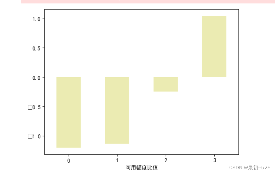
4.3 WOE 随机查看
cut1_woe.plot.bar(color='y',alpha=0.3,rot=0)
4.4 IV值的计算
# 可以看出woe已调整到具有单调性
# **3、IV值计算**```
def get_IV_data(cut,cut_woe):
    grouped=data["好坏客户"].groupby(cut,as_index = True).value_counts()
    cut_IV=((grouped.unstack().iloc[:,1]/data["好坏客户"].sum()-grouped.unstack().iloc[:,0]/(data["好坏客户"].count()-data["好坏客户"].sum()))*cut_woe).sum()
    return cut_IV
#计算各分组的IV值
cut1_IV=get_IV_data(cut1,cut1_woe)
cut2_IV=get_IV_data(cut2,cut2_woe)
cut3_IV=get_IV_data(cut3,cut3_woe)
cut4_IV=get_IV_data(cut4,cut4_woe)
cut5_IV=get_IV_data(cut5,cut5_woe)
cut6_IV=get_IV_data(cut6,cut6_woe)
cut7_IV=get_IV_data(cut7,cut7_woe)
cut8_IV=get_IV_data(cut8,cut8_woe)
cut9_IV=get_IV_data(cut9,cut9_woe)
cut10_IV=get_IV_data(cut10,cut10_woe)
IV=pd.DataFrame([cut1_IV,cut2_IV,cut3_IV,cut4_IV,cut5_IV,cut6_IV,cut7_IV,cut8_IV,cut9_IV,cut10_IV],index=['可用额度比值','年龄','逾期30-59天笔数','负债率','月收入','信贷数量','逾期90天笔数','固定资产贷款量','逾期60-89天笔数','家属数量'],columns=['IV'])
iv=IV.plot.bar(color='y',alpha=0.3,rot=30,figsize=(10,5),fontsize=(10))
iv.set_title('特征变量与IV值分布图',fontsize=(15))
iv.set_xlabel('特征变量',fontsize=(15))
iv.set_ylabel('IV',fontsize=(15))
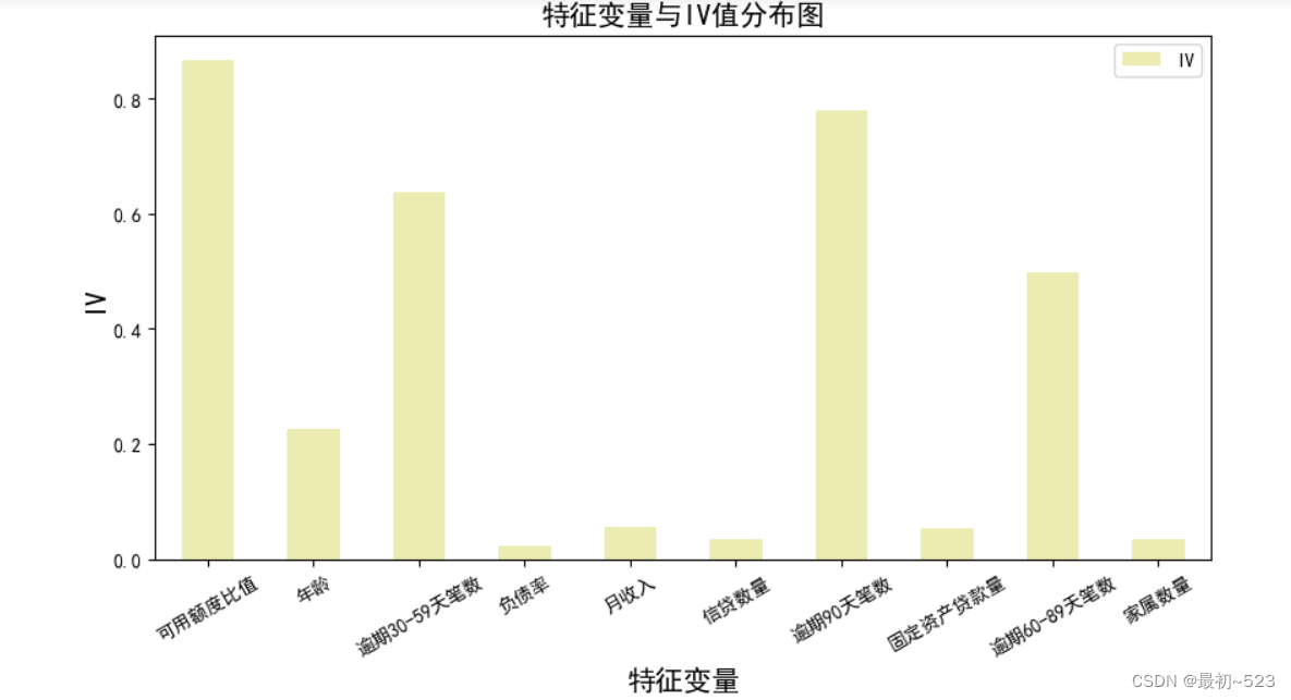
4.5 IV值计算的查看 IV值大于0.02即可以作为预测值进行预测
IV

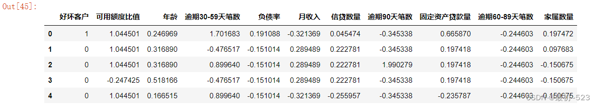
4.6 WOE值的替换
df_new=pd.DataFrame() #新建df_new存放woe转换后的数据
def replace_data(cut,cut_woe):
    a=[]
    for i in cut.unique():
        a.append(i)
        a.sort()
    for m in range(len(a)):
        cut.replace(a[m],cut_woe.values[m],inplace=True)
    return cut
df_new['好坏客户']=data['好坏客户']
df_new['可用额度比值']=replace_data(cut1,cut1_woe)
df_new['年龄']=replace_data(cut2,cut2_woe)
df_new['逾期30-59天笔数']=replace_data(cut3,cut3_woe)
df_new['负债率']=replace_data(cut4,cut4_woe)
df_new['月收入']=replace_data(cut5,cut5_woe)
df_new['信贷数量']=replace_data(cut6,cut6_woe)
df_new['逾期90天笔数']=replace_data(cut7,cut7_woe)
df_new['固定资产贷款量']=replace_data(cut8,cut8_woe)
df_new['逾期60-89天笔数']=replace_data(cut9,cut9_woe)
df_new['家属数量']=replace_data(cut10,cut10_woe)
df_new.head()
4.7 计算字段之间的相关性
import seaborn as sns
corr = data.corr()#计算各变量的相关性系数
xticks = list(corr.index)#x轴标签
yticks = list(corr.index)#y轴标签
fig = plt.figure(figsize=(20,10))
ax1 = fig.add_subplot(1, 1, 1)
sns.heatmap(corr, annot=True, cmap="rainbow",ax=ax1,linewidths=.5, annot_kws={'size': 20, 'weight': 'bold', 'color': 'yellow'})
ax1.set_xticklabels(xticks, rotation=90, fontsize=25)
ax1.set_yticklabels(yticks, rotation=0, fontsize=20)
plt.show()
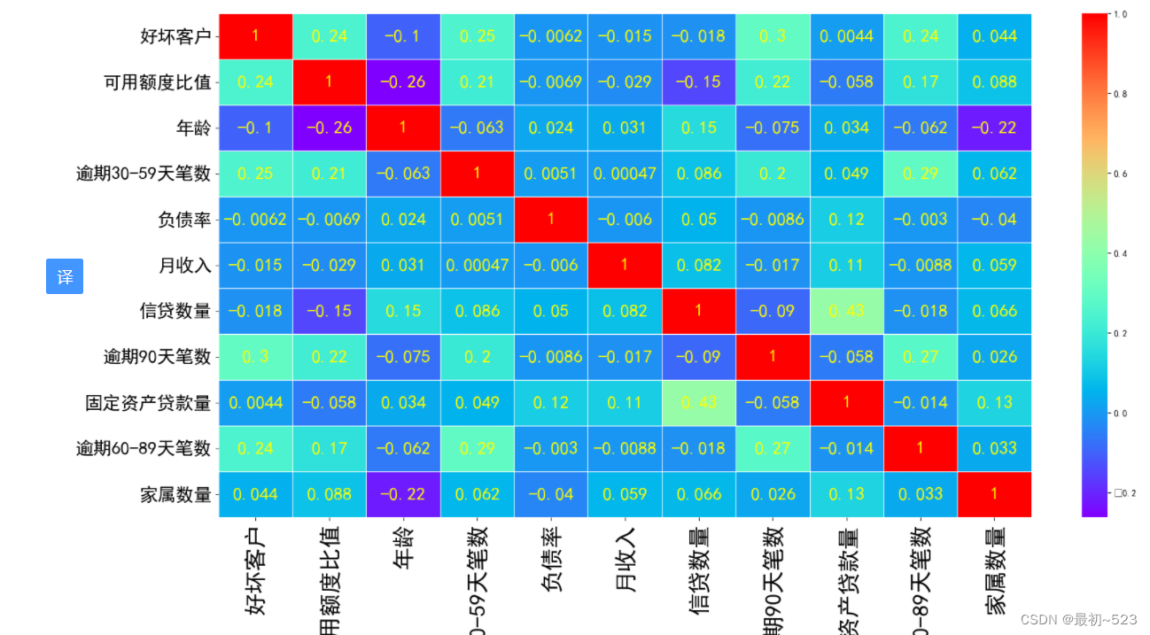
由上面相关性可以看出可以看到各变量之间的相关性比较小,所以不需要操作,一般相关系数大于0.6可以进行变量剔除
5.建模评估
导入机器学习库,并根据前面的IV和相关性 剔除掉几乎没有预测能力的字段
from sklearn.linear_model import LogisticRegression
from sklearn.model_selection import train_test_split
train=df_new.drop(["负债率","月收入","信贷数量","固定资产贷款量","家属数量"],axis=1)
train.head()
第一种 建立逻辑回归模型
5.1 建立模型进行预测
x=train.iloc[:,1:] #设定自变量
y=train.iloc[:,0] #设定因变量

#将数据集进行切割,分成训练集和测试集,其中样本占比0.8,采用随机抽样
train_x,test_x,train_y,test_y=train_test_split(x,y,test_size=0.2,random_state=4)

#建立模型
model=LogisticRegression()
result=model.fit(train_x,train_y) #训练模型,将结果保存为result
pred_y=model.predict(test_x)  #预测测试集的y
result.score(test_x,test_y)    #计算预测精度 正确率
0.9415859988776656
y_pred = model.predict(test_x)
y_pred[:500]
array([0, 0, 0, 0, 0, 0, 0, 0, 0, 0, 0, 0, 0, 0, 0, 0, 0, 0, 0, 0, 0, 0,
       0, 0, 0, 0, 0, 1, 0, 0, 0, 0, 0, 0, 0, 0, 0, 0, 0, 0, 0, 0, 0, 0,
       0, 0, 0, 0, 0, 0, 0, 0, 0, 0, 0, 1, 0, 0, 0, 0, 0, 0, 0, 0, 0, 0,
       0, 0, 0, 0, 0, 0, 0, 0, 0, 1, 0, 0, 0, 0, 0, 0, 0, 0, 0, 0, 0, 0,
       0, 0, 0, 0, 0, 0, 0, 0, 0, 0, 0, 0, 0, 0, 0, 0, 0, 0, 0, 0, 1, 0,
       0, 0, 0, 0, 0, 0, 0, 0, 0, 0, 0, 0, 0, 0, 0, 0, 0, 0, 0, 0, 0, 0,
       0, 0, 0, 0, 0, 0, 0, 0, 0, 0, 0, 0, 0, 0, 0, 0, 0, 0, 0, 0, 0, 0,
       0, 0, 0, 0, 0, 0, 0, 0, 0, 0, 0, 0, 0, 0, 0, 0, 0, 0, 0, 0, 0, 0,
       0, 0, 0, 0, 0, 0, 0, 0, 0, 0, 0, 0, 0, 0, 0, 0, 0, 0, 0, 0, 0, 0,
       0, 0, 0, 0, 0, 0, 0, 0, 0, 0, 0, 0, 0, 0, 0, 0, 0, 0, 0, 0, 0, 0,
       0, 0, 0, 0, 0, 0, 0, 0, 0, 0, 0, 0, 0, 0, 0, 0, 0, 0, 0, 0, 0, 0,
       0, 0, 0, 0, 0, 0, 0, 0, 0, 0, 0, 1, 0, 0, 0, 0, 0, 0, 0, 0, 0, 0,
       0, 0, 0, 0, 0, 0, 0, 0, 0, 0, 0, 0, 0, 0, 0, 0, 0, 0, 0, 0, 0, 0,
       0, 1, 0, 0, 0, 0, 0, 0, 0, 0, 0, 0, 0, 0, 0, 0, 0, 0, 0, 0, 0, 0,
       0, 0, 0, 0, 0, 0, 0, 0, 0, 0, 0, 0, 0, 0, 0, 0, 0, 0, 0, 0, 0, 0,
       0, 0, 0, 0, 0, 1, 0, 0, 0, 0, 0, 0, 0, 0, 0, 0, 0, 0, 0, 0, 0, 0,
       0, 0, 0, 0, 0, 0, 0, 0, 0, 0, 0, 0, 0, 0, 0, 0, 0, 0, 0, 0, 0, 0,
       0, 0, 0, 0, 0, 0, 0, 0, 0, 0, 0, 0, 0, 0, 0, 0, 0, 0, 0, 0, 0, 0,
       0, 0, 0, 0, 0, 0, 0, 0, 0, 0, 0, 0, 0, 0, 0, 0, 0, 0, 0, 0, 0, 0,
       0, 0, 0, 0, 0, 0, 0, 0, 0, 0, 0, 0, 0, 0, 0, 0, 0, 0, 0, 0, 0, 0,
       0, 0, 0, 0, 0, 0, 0, 0, 0, 0, 0, 0, 0, 0, 0, 0, 0, 0, 0, 0, 0, 0,
       0, 0, 0, 0, 0, 0, 0, 0, 0, 0, 0, 0, 0, 0, 0, 0, 0, 0, 0, 0, 0, 0,
       0, 0, 0, 0, 0, 0, 0, 0, 0, 0, 0, 0, 0, 0, 0, 0], dtype=int64)
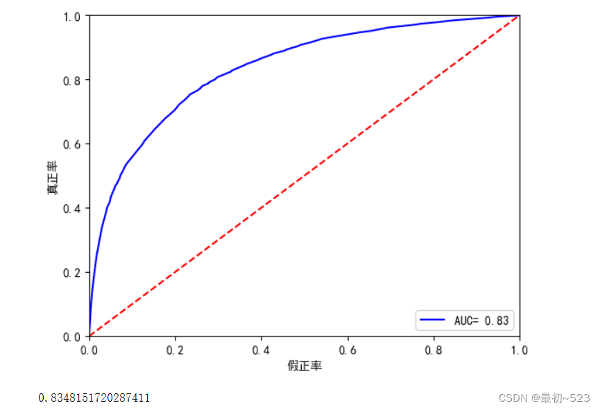
5.2利用sklearn.metrics计算ROC和AUC值
from sklearn.metrics import  roc_curve, auc  #导入函数
proba_y=model.predict_proba(test_x)  #预测概率predict_proba:
'''返回的是一个n行k列的数组,第i行第j列上的数值是模型预测第i个预测样本的标签为j的概率,此时每一行的和应该等于1。'''
fpr,tpr,threshold=roc_curve(test_y,proba_y[:,1])  #计算threshold阈值,tpr真正例率,fpr假正例率,大于阈值的视为1即坏客户
roc_auc=auc(fpr,tpr)   #计算AUC值

plt.plot(fpr,tpr,'b',label= 'AUC= %0.2f' % roc_auc) #生成roc曲线
plt.legend(loc='lower right')
plt.plot([0,1],[0,1],'r--')
plt.xlim([0,1])
plt.ylim([0,1])
plt.ylabel('真正率')
plt.xlabel('假正率')
plt.show()
print(roc_auc)
5.3 ks曲线评估
fig, ax = plt.subplots()
ax.plot(1 - threshold, tpr, label='tpr') # ks曲线要按照预测概率降序排列,所以需要1-threshold镜像
ax.plot(1 - threshold, fpr, label='fpr')
ax.plot(1 - threshold, tpr-fpr,label='KS')
plt.xlabel('score')
plt.title('KS Curve')
plt.ylim([0.0, 1.0])
plt.figure(figsize=(20,20))
legend = ax.legend(loc='upper left')
plt.show()
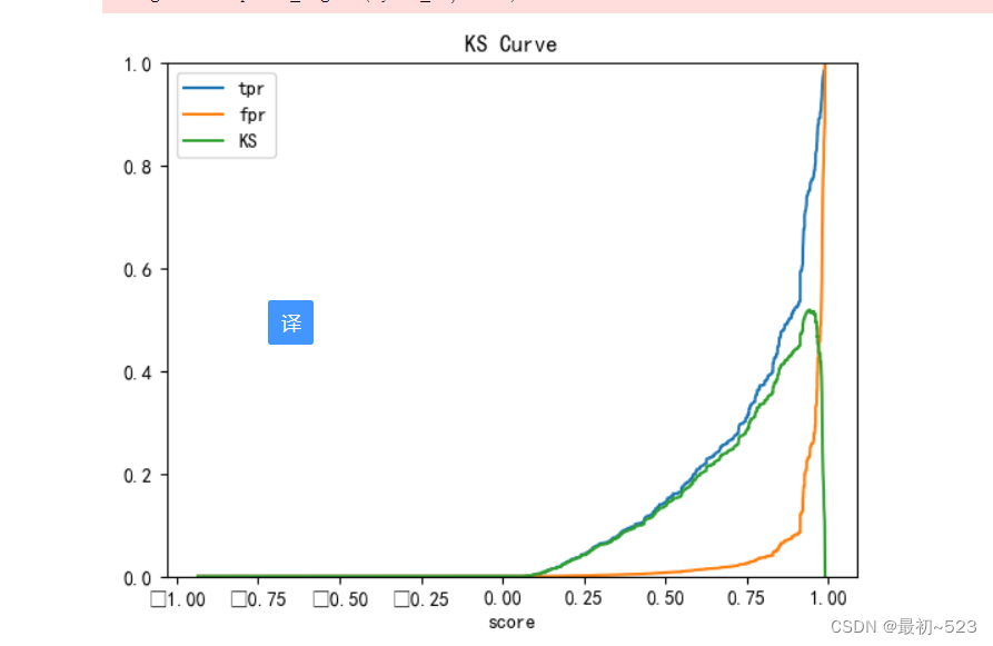
max(tpr-fpr)
0.5192829989663486
5.4 召回率
from sklearn.metrics import recall_score
recall = recall_score(test_y, pred_y)
print("Recall:", recall)
Recall: 0.1445432026810433
第二种 随机森林模型及进行预测
5.1 导入模型库 数据划分 进行预测
import numpy as np
from sklearn.model_selection import train_test_split
from sklearn.metrics import accuracy_score,recall_score,precision_score
from sklearn.ensemble import RandomForestClassifier


# 划分训练集和测试集
X_train, X_test, y_train, y_test = train_test_split(x, y, test_size=0.2, random_state=42)

# 建立随机森林模型
rfc = RandomForestClassifier(random_state=42, n_estimators=100)
rfc.fit(X_train, y_train)

# 模型评估
y_pred = rfc.predict(X_test)
print('准确率: ', accuracy_score(y_test, y_pred))
print('精确率: ', precision_score(y_test, y_pred))
print('召回率: ', recall_score(y_test, y_pred))
准确率:  0.9456719977553311
精确率:  0.6761133603238867
召回率:  0.1491515331944031
模型的评估属于一般 召回率不是很好 ,问题可能为数据的不均衡


 被折叠的 条评论
为什么被折叠?
被折叠的 条评论
为什么被折叠?
 到【灌水乐园】发言


