机器学习-特征选择-序列后向选择Sequential Backward Selection方法

Section I: Brief Introduction on Sequential Backward Selection方法

The idea behind the SBS algorithm is quite simple: SBS sequentially removes features from the full feature subset until new feature subspace contains the desired number of features. In order to determine which feature is to be removed at each stage, we need to define the criterion function J that we want to minimize.The criterion calculated by the criterion function can simply be the difference in performance of the classifier before and after the removal of a particular feature. Then, the feature to be removed at each stage can simply be defined as the feature that maximizes this criterion;or in more intuitive terms,at each stage we eliminate the feature that causes the least performance loss after removal.
Personal Views:

1. 每一步依据当前特征组合，选择模型训练泛化性能最佳者
2. 下一步的特征组合是前一步特征空间的子集

From
Sebastian Raschka, Vahid Mirjalili. Python机器学习第二版. 南京：东南大学出版社，2018.

Section II: Code Implementation and Feature Selection

第一部分：Code Bundle of Sequential Backward Selection

from sklearn.base import clone
from itertools import combinations
import numpy as np
from sklearn.metrics import accuracy_score
from sklearn.model_selection import train_test_split

class SBS():
    def __init__(self,estimator,k_features,
                 scoring=accuracy_score,
                 test_size=0.25,random_state=1):
        self.scoring=scoring
        self.estimator=clone(estimator)
        self.k_features=k_features
        self.test_size=test_size
        self.random_state=random_state

    def fit(self,X,y):
        X_train,X_test,y_train,y_test=\
            train_test_split(X,y,test_size=self.test_size,random_state=self.random_state)
        dim=X_train.shape[1]
        self.indices_=tuple(range(dim))
        self.subsets_=[self.indices_]
        score=self._calc_score(X_train,y_train,X_test,y_test,self.indices_)
        self.scores_=[score]

        while dim>self.k_features:
            scores=[]
            subsets=[]

            for p in combinations(self.indices_,r=dim-1):
                score=self._calc_score(X_train,y_train,X_test,y_test,p)
                scores.append(score)
                subsets.append(p)

            best=np.argmax(scores)
            self.indices_=subsets[best]
            self.subsets_.append(self.indices_)
            dim-=1

            self.scores_.append(scores[best])
        self.k_score_=self.scores_[-1]
        return self

    def transform(self,X,y):
        return X[:,self.indices_]

    def _calc_score(self,X_train,y_train,X_test,y_test,indices):
        self.estimator.fit(X_train[:,indices],y_train)
        y_pred=self.estimator.predict(X_test[:,indices])
        score=self.scoring(y_test,y_pred)
        return score

第二部分：调用方式-主函数

import matplotlib.pyplot as plt
from sklearn import datasets
from sklearn.preprocessing import StandardScaler
from sklearn.model_selection import train_test_split
import numpy as np
from sklearn.neighbors import KNeighborsClassifier
from SequentialBackwardSelection import sequentialbackwardselection

#Section 1: Prepare data
plt.rcParams['figure.dpi']=200
plt.rcParams['savefig.dpi']=200
font = {'family': 'Times New Roman',
        'weight': 'light'}
plt.rc("font", **font)

#Section 1: Load data and split it into train/test dataset
wine=datasets.load_wine()
X,y=wine.data,wine.target
X_train,X_test,y_train,y_test=train_test_split(X,y,test_size=0.3,random_state=1,stratify=y)

#Section 2: Standardize data
sc=StandardScaler()
sc.fit(X_train)
X_train_std=sc.transform(X_train)
X_test_std=sc.transform(X_test)

#Section 3: Feature Selection Via SBS
knn=KNeighborsClassifier(n_neighbors=5)
sbs=sequentialbackwardselection.SBS(knn,k_features=1)
sbs.fit(X_train_std,y_train)

#Section 4: Visualize the trend of model performance versus feature numbers
k_feat=[len(k) for k in sbs.subsets_]
plt.plot(k_feat,sbs.scores_,marker='o')
plt.ylim([0.7,1.02])
plt.ylabel('Accuracy')
plt.xlabel('Feature Numbers')
plt.grid()
plt.savefig('./fig1.png')
plt.show()

第三部分：运行结果：

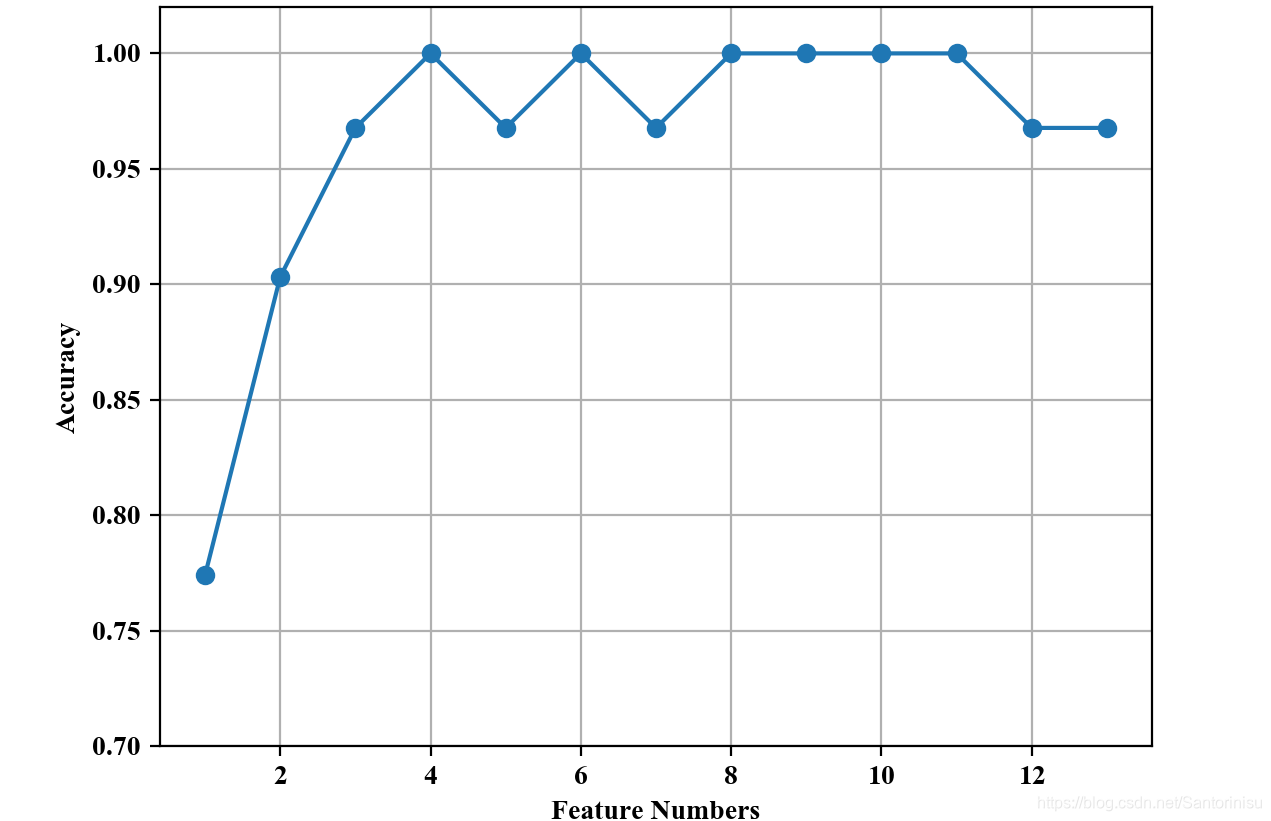
由上图可以得知，显然初始特征量并不是最佳，有可能部分特征是冗余的，也会给模型最佳训练方向带来干扰。因此，适当的特征选择也是必要的。

参考文献：
Sebastian Raschka, Vahid Mirjalili. Python机器学习第二版. 南京：东南大学出版社，2018.