


版权声明:本套技术专栏是作者(秦凯新)平时工作的总结和升华,通过从真实商业环境抽取案例进行总结和分享,并给出商业应用的调优建议和集群环境容量规划等内容,请持续关注本套博客。QQ邮箱地址:1120746959@qq.com,如有任何学术交流,可随时联系。

1 Numpy详细使用
-
读取txt文件
import numpy world_alcohol = numpy.genfromtxt("world_alcohol.txt", delimiter=",") print(type(world_alcohol)) world_alcohol = numpy.genfromtxt("world_alcohol.txt", delimiter=",", dtype="U75", skip_header=1) print(world_alcohol) [[u'1986' u'Western Pacific' u'Viet Nam' u'Wine' u'0'] [u'1986' u'Americas' u'Uruguay' u'Other' u'0.5'] [u'1985' u'Africa' u"Cte d'Ivoire" u'Wine' u'1.62'] ..., [u'1987' u'Africa' u'Malawi' u'Other' u'0.75'] [u'1989' u'Americas' u'Bahamas' u'Wine' u'1.5'] [u'1985' u'Africa' u'Malawi' u'Spirits' u'0.31']] -
创建一维和二维的Array数组
#The numpy.array() function can take a list or list of lists as input. When we input a list, we get a one-dimensional array as a result: #一维的Array数组[] vector = numpy.array([5, 10, 15, 20]) #二维的Array数组[[],[],[]] matrix = numpy.array([[5, 10, 15], [20, 25, 30], [35, 40, 45]]) print vector print matrix -
shape用法
#We can use the ndarray.shape property to figure out how many elements are in the array vector = numpy.array([1, 2, 3, 4]) print(vector.shape) #For matrices, the shape property contains a tuple with 2 elements. matrix = numpy.array([[5, 10, 15], [20, 25, 30]]) print(matrix.shape) (4,) (2, 3) -
dtype用法(numpy要求numpy.array内部元素结构相同)
numbers = numpy.array([1, 2, 3, 4]) numbers.dtype dtype('int32') #改变其中一个值时,其他值都会改变 numbers = numpy.array([1, 2, 3, '4']) print(numbers) numbers.dtype ['1' '2' '3' '4'] dtype('<U11') -
索引定位
[[u'1986' u'Western Pacific' u'Viet Nam' u'Wine' u'0'] [u'1986' u'Americas' u'Uruguay' u'Other' u'0.5'] [u'1985' u'Africa' u"Cte d'Ivoire" u'Wine' u'1.62'] ..., [u'1987' u'Africa' u'Malawi' u'Other' u'0.75'] [u'1989' u'Americas' u'Bahamas' u'Wine' u'1.5'] [u'1985' u'Africa' u'Malawi' u'Spirits' u'0.31']] uruguay_other_1986 = world_alcohol[1,4] third_country = world_alcohol[2,2] print uruguay_other_1986 print third_country 0.5 Cte d'Ivoire -
索引切片
vector = numpy.array([5, 10, 15, 20]) print(vector[0:3]) [ 5 10 15] -
取某一列(:表示所有行)
matrix = numpy.array([ [5, 10, 15], [20, 25, 30], [35, 40, 45] ]) print(matrix[:,1]) [10 25 40] matrix = numpy.array([ [5, 10, 15], [20, 25, 30], [35, 40, 45] ]) print(matrix[:,0:2]) [[ 5 10] [20 25] [35 40]] matrix = numpy.array([ [5, 10, 15], [20, 25, 30], [35, 40, 45] ]) print(matrix[1:3,0:2]) [[20 25] [35 40]] -
对Array操作表示对内部所有元素进行操作
import numpy #it will compare the second value to each element in the vector # If the values are equal, the Python interpreter returns True; otherwise, it returns False vector = numpy.array([5, 10, 15, 20]) vector == 10 array([False, True, False, False], dtype=bool) matrix = numpy.array([ [5, 10, 15], [20, 25, 30], [35, 40, 45] ]) matrix == 25 array([[False, False, False], [False, True, False], [False, False, False]], dtype=bool) -
布尔值当索引([False True False False])
vector = numpy.array([5, 10, 15, 20]) equal_to_ten = (vector == 10) print equal_to_ten print(vector[equal_to_ten]) [False True False False] [10] #矩阵表示索引 matrix = numpy.array([ [5, 10, 15], [20, 25, 30], [35, 40, 45] ]) second_column_25 = (matrix[:,1] == 25) print second_column_25 print(matrix[second_column_25, :]) [False True False] [[20 25 30]] -
对数组进行与运算
#We can also perform comparisons with multiple conditions vector = numpy.array([5, 10, 15, 20]) equal_to_ten_and_five = (vector == 10) & (vector == 5) print equal_to_ten_and_five [False False False False] vector = numpy.array([5, 10, 15, 20]) equal_to_ten_or_five = (vector == 10) | (vector == 5) print equal_to_ten_or_five [ True True False False] -
值类型转换
vector = numpy.array(["1", "2", "3"]) print vector.dtype print vector vector = vector.astype(float) print vector.dtype print vector |S1 ['1' '2' '3'] float64 [ 1. 2. 3.] -
聚合求解
vector = numpy.array([5, 10, 15, 20]) vector.sum() -
按行维度(axis=1)
matrix = numpy.array([ [5, 10, 15], [20, 25, 30], [35, 40, 45] ]) matrix.sum(axis=1) array([ 30, 75, 120]) -
按列求和(axis=0)
matrix = numpy.array([ [5, 10, 15], [20, 25, 30], [35, 40, 45] ]) matrix.sum(axis=0) array([60, 75, 90]) -
矩阵操作np.arange生成0-N的整数
import numpy as np a = np.arange(15).reshape(3, 5) a array([[ 0, 1, 2, 3, 4], [ 5, 6, 7, 8, 9], [10, 11, 12, 13, 14]]) a.ndim 2 a.dtype.name 'int32' a.size 15 -
矩阵初始化
np.zeros ((3,4)) array([[ 0., 0., 0., 0.], [ 0., 0., 0., 0.], [ 0., 0., 0., 0.]]) np.ones( (2,3,4), dtype=np.int32 ) array([[[1, 1, 1, 1], [1, 1, 1, 1], [1, 1, 1, 1]], [[1, 1, 1, 1], [1, 1, 1, 1], [1, 1, 1, 1]]]) -
按照间隔生成数据
np.arange( 10, 30, 5 ) array([10, 15, 20, 25]) np.arange( 0, 2, 0.3 ) array([ 0. , 0.3, 0.6, 0.9, 1.2, 1.5, 1.8]) -
随机生成数据
np.random.random((2,3)) array([[ 0.40130659, 0.45452825, 0.79776512], [ 0.63220592, 0.74591134, 0.64130737]]) -
linspace在0到2pi之间取100个数
from numpy import pi np.linspace( 0, 2*pi, 100 ) array([ 0. , 0.06346652, 0.12693304, 0.19039955, 0.25386607, 0.31733259, 0.38079911, 0.44426563, 0.50773215, 0.57119866, 0.63466518, 0.6981317 , 0.76159822, 0.82506474, 0.88853126, 0.95199777, 1.01546429, 1.07893081, 1.14239733, 1.20586385, 1.26933037, 1.33279688, 1.3962634 , 1.45972992, 1.52319644, 1.58666296, 1.65012947, 1.71359599, 1.77706251, 1.84052903, 1.90399555, 1.96746207, 2.03092858, 2.0943951 , 2.15786162, 2.22132814, 2.28479466, 2.34826118, 2.41172769, 2.47519421, 2.53866073, 2.60212725, 2.66559377, 2.72906028, 2.7925268 , 2.85599332, 2.91945984, 2.98292636, 3.04639288, 3.10985939, 3.17332591, 3.23679243, 3.30025895, 3.36372547, 3.42719199, 3.4906585 , 3.55412502, 3.61759154, 3.68105806, 3.74452458, 3.8079911 , 3.87145761, 3.93492413, 3.99839065, 4.06185717, 4.12532369, 4.1887902 , 4.25225672, 4.31572324, 4.37918976, 4.44265628, 4.5061228 , 4.56958931, 4.63305583, 4.69652235, 4.75998887, 4.82345539, 4.88692191, 4.95038842, 5.01385494, 5.07732146, 5.14078798, 5.2042545 , 5.26772102, 5.33118753, 5.39465405, 5.45812057, 5.52158709, 5.58505361, 5.64852012, 5.71198664, 5.77545316, 5.83891968, 5.9023862 , 5.96585272, 6.02931923, 6.09278575, 6.15625227, 6.21971879, 6.28318531]) -
矩阵基本操作
#the product operator * operates elementwise in NumPy arrays a = np.array( [20,30,40,50] ) b = np.arange( 4 ) print (a) print (b) #b c = a-b print (c) b**2 print (b**2) print (a<35) [20 30 40 50] [0 1 2 3] [20 29 38 47] [ True True False False] -
矩阵相乘
#The matrix product can be performed using the dot function or method A = np.array([[1,1], [0,1]] ) B = np.array([[2,0], [3,4]]) print (A) print (B) print (A*B) print (A.dot(B)) print (np.dot(A, B) ) [[1 1] [0 1]] [[2 0] [3 4]] [[2 0] [0 4]] [[5 4] [3 4]] [[5 4] [3 4]] -
矩阵操作floor向下取整
import numpy as np B = np.arange(3) print (B) #print np.exp(B) print (np.sqrt(B)) [0 1 2] [0. 1. 1.41421356] #Return the floor of the input a = np.floor(10*np.random.random((3,4))) #print a #Return the floor of the input a = np.floor(10*np.random.random((3,4))) print (a) print(a.reshape(2,-1)) [[0. 4. 2. 2.] [8. 1. 5. 7.] [0. 9. 7. 4.]] [[0. 4. 2. 2. 8. 1.] [5. 7. 0. 9. 7. 4.]] -
hstack矩阵拼接
a = np.floor(10*np.random.random((2,2))) b = np.floor(10*np.random.random((2,2))) print a print '---' print b print '---' print np.hstack((a,b)) [[ 5. 6.] [ 1. 5.]] --- [[ 8. 6.] [ 9. 0.]] --- [[ 5. 6. 8. 6.] [ 1. 5. 9. 0.]] a = np.floor(10*np.random.random((2,2))) b = np.floor(10*np.random.random((2,2))) print (a) print ('---') print (b) print ('---') #print np.hstack((a,b)) np.vstack((a,b)) [[7. 7.] [2. 6.]] --- [[0. 6.] [0. 3.]] --- array([[1., 0.], [3., 6.], [4., 2.], [8., 7.]]) a = np.floor(10*np.random.random((2,12))) print (a) print (np.hsplit(a,3)) [[6. 5. 2. 4. 2. 4. 9. 4. 4. 6. 8. 9.] [8. 4. 0. 2. 6. 5. 2. 5. 0. 4. 1. 6.]] [array([[6., 5., 2., 4.], [8., 4., 0., 2.]]), array([[2., 4., 9., 4.], [6., 5., 2., 5.]]), array([[4., 6., 8., 9.], [0., 4., 1., 6.]])] -
任意选择切分位置
print ( np.hsplit(a,(3,4))) # Split a after the third and the fourth column [[2. 8. 4. 7. 6. 6. 5. 8. 8. 3. 0. 1.] [3. 5. 9. 4. 5. 8. 7. 6. 2. 3. 8. 4.]] [array([[2., 8., 4.], [3., 5., 9.]]), array([[7.], [4.]]), array([[6., 6., 5., 8., 8., 3., 0., 1.], [5., 8., 7., 6., 2., 3., 8., 4.]])] -
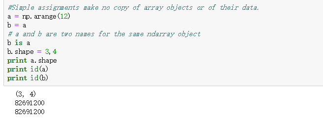
变量赋值
-
变量视图
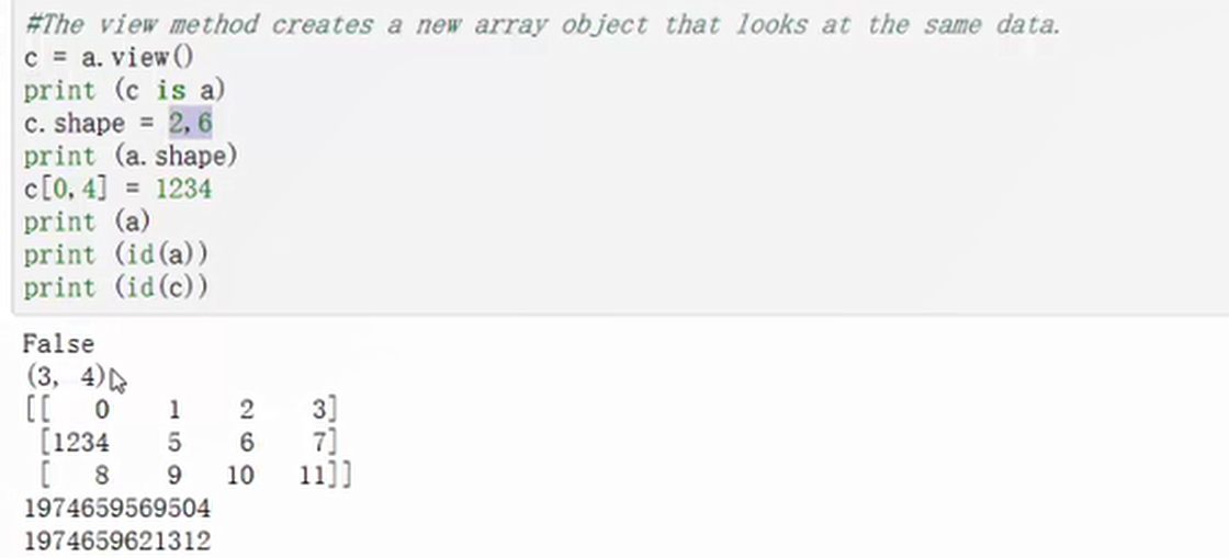
-
copy实现变量之间没有关系
d = a.copy() d is a d[0,0] = 9999 print d print a [[9999 1 2 3] [1234 5 6 7] [ 8 9 10 11]] [[ 0 1 2 3] [1234 5 6 7] [ 8 9 10 11]] -
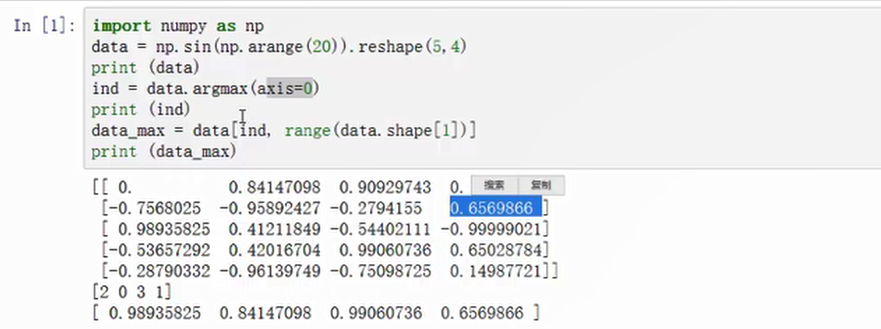
寻找列最大值索引
-
行列按照倍数扩展(行3倍列5倍)
a = np.arange(0, 40, 10) b = np.tile(a, (3, 5)) print b [[ 0 10 20 30 0 10 20 30 0 10 20 30 0 10 20 30 0 10 20 30] [ 0 10 20 30 0 10 20 30 0 10 20 30 0 10 20 30 0 10 20 30] [ 0 10 20 30 0 10 20 30 0 10 20 30 0 10 20 30 0 10 20 30]] -
按照元素大小排序并给出索引值
a = np.array([4, 3, 1, 2]) j = np.argsort(a) print j print a[j] [2 3 1 0] [1 2 3 4] -
对数组按照元素大小排序
  a = np.array([[4, 3, 5], [1, 2, 1]])
  #print a
  b = np.sort(a, axis=1)
  print (b)

  [[3 4 5]
  [1 1 2]]
2 Pandas详细使用(底层基于Numpy)
2.1 Pandas基本操作
- Pandas核心结构(DataFrame)
- Pandas 字符型表示为Object
- Pandas数据基本类型展示
import pandas
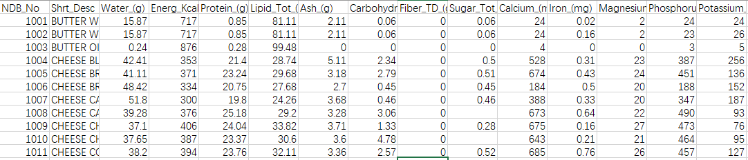
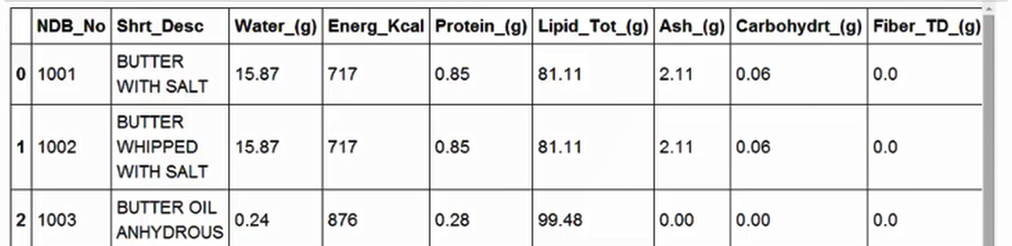
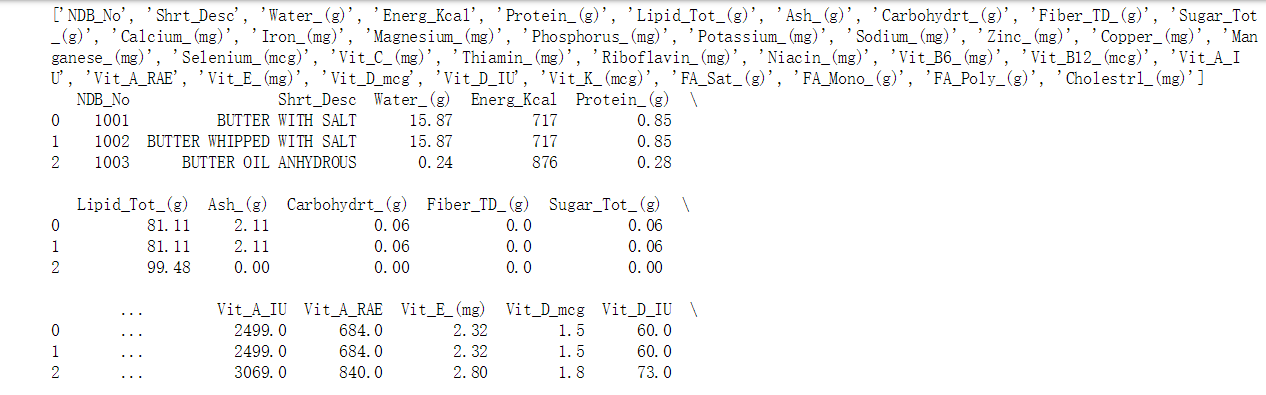
food_info = pandas.read_csv("food_info.csv")
print(type(food_info))
<class 'pandas.core.frame.DataFrame'>
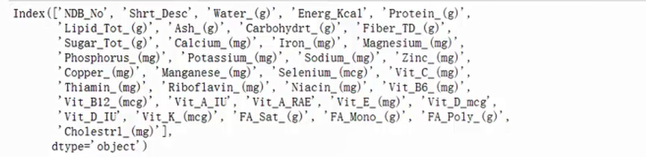
col_names = food_info.columns.tolist()
['NDB_No', 'Shrt_Desc', 'Water_(g)', 'Energ_Kcal', 'Protein_(g)', 'Lipid_Tot_(g)', 'Ash_(g)',
'Carbohydrt_(g)', 'Fiber_TD_(g)', 'Sugar_Tot_(g)', 'Calcium_(mg)', 'Iron_(mg)',
'Magnesium_(mg)', 'Phosphorus_(mg)', 'Potassium_(mg)', 'Sodium_(mg)', 'Zinc_(mg)',
'Copper_(mg)', 'Manganese_(mg)', 'Selenium_(mcg)', 'Vit_C_(mg)', 'Thiamin_(mg)',
'Riboflavin_(mg)', 'Niacin_(mg)', 'Vit_B6_(mg)', 'Vit_B12_(mcg)', 'Vit_A_IU', 'Vit_A_RAE',
'Vit_E_(mg)', 'Vit_D_mcg', 'Vit_D_IU', 'Vit_K_(mcg)', 'FA_Sat_(g)', 'FA_Mono_(g)',
'FA_Poly_(g)', 'Cholestrl_(mg)']
print food_info.dtypes
NDB_No int64
Shrt_Desc object
Water_(g) float64
Energ_Kcal int64
Protein_(g) float64
Lipid_Tot_(g) float64
Ash_(g) float64
Carbohydrt_(g) float64
Fiber_TD_(g) float64
Sugar_Tot_(g) float64
Calcium_(mg) float64
Iron_(mg) float64
Magnesium_(mg) float64
Phosphorus_(mg) float64
Potassium_(mg) float64
Sodium_(mg) float64
Zinc_(mg) float64
Copper_(mg) float64
Manganese_(mg) float64
Selenium_(mcg) float64
Vit_C_(mg) float64
Thiamin_(mg) float64
Riboflavin_(mg) float64
Niacin_(mg) float64
Vit_B6_(mg) float64
Vit_B12_(mcg) float64
Vit_A_IU float64
Vit_A_RAE float64
Vit_E_(mg) float64
Vit_D_mcg float64
Vit_D_IU float64
Vit_K_(mcg) float64
FA_Sat_(g) float64
FA_Mono_(g) float64
FA_Poly_(g) float64
Cholestrl_(mg) float64
dtype: object
-
Pandas基本操作
  #可以指定数量
  #first_rows = food_info.head()
  #print(food_info.head(3))
#print food_info.columns
    #print food_info.shape
    (8618,36)
-
取数据操作
#pandas uses zero-indexing #Series object representing the row at index 0. #print food_info.loc[0] # Series object representing the seventh row. #food_info.loc[6] # Will throw an error: "KeyError: 'the label [8620] is not in the [index]'" #food_info.loc[8620] #The object dtype is equivalent to a string in Python -
数据切片
# Returns a DataFrame containing the rows at indexes 3, 4, 5, and 6. #food_info.loc[3:6] # Returns a DataFrame containing the rows at indexes 2, 5, and 10. Either of the following approaches will work. # Method 1 #two_five_ten = [2,5,10] #food_info.loc[two_five_ten] # Method 2 #food_info.loc[[2,5,10]] -
通过列名取出数据
  # Series object representing the "NDB_No" column.
  #ndb_col = food_info["NDB_No"]
  #print ndb_col
  # Alternatively, you can access a column by passing in a string variable.
  #col_name = "NDB_No"
  #ndb_col = food_info[col_name]
-
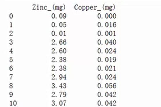
取出两个列的值
  #columns = ["Zinc_(mg)", "Copper_(mg)"]
  #zinc_copper = food_info[columns]
  #print zinc_copper
  #print zinc_copper
  # Skipping the assignment.
  #zinc_copper = food_info[["Zinc_(mg)", "Copper_(mg)"]]
-
endswith 定位取值
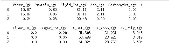
  #print(food_info.columns)
  #print(food_info.head(2))
  col_names = food_info.columns.tolist()
  #print col_names
  gram_columns = []

  for c in col_names:
      if c.endswith("(g)"):
          gram_columns.append(c)
  gram_df = food_info[gram_columns]
  print(gram_df.head(3))
2.2 Series类型上场
Series 是一个带有 名称 和索引的一维数组,既然是数组,肯定要说到的就是数组中的元素类型,在 Series 中包含的数据类型可以是整数、浮点、字符串、Python对象等。
    # 存储了 4 个年龄:18/30/25/40
    user_age = pd.Series(data=[18, 30, 25, 40])
    user_age

    0    18
    1    30
    2    25
    3    40
    dtype: int64
-
指定索引
user_age.index = ["Tom", "Bob", "Mary", "James"] user_age Tom 18 Bob 30 Mary 25 James 40 dtype: int64 -
为 index 起个名字
user_age.index.name = "name" user_age name Tom 18 Bob 30 Mary 25 James 40 dtype: int64 -
给 Series 起个名字
user_age.name="user_age_info" user_age name Tom 18 Bob 30 Mary 25 James 40 Name: user_age_info, dtype: int64 -
一个 Series 包括了 data、index 以及 name。
# 构建索引 name = pd.Index(["Tom", "Bob", "Mary", "James"], name="name") # 构建 Series user_age = pd.Series(data=[18, 30, 25, 40], index=name, name="user_age_info") user_age name Tom 18 Bob 30 Mary 25 James 40 Name: user_age_info, dtype: int64 # 指定类型为浮点型 user_age = pd.Series(data=[18, 30, 25, 40], index=name, name="user_age_info", dtype=float) user_age name Tom 18.0 Bob 30.0 Mary 25.0 James 40.0 Name: user_age_info, dtype: float64 -
Series 包含了 dict 的特点,也就意味着可以使用与 dict 类似的一些操作。我们可以将 index 中的元素看成是 dict 中的 key。
 # 获取 Tom 的年龄
  user_age["Tom"]

  18.0

  user_age.get("Tom")
  18.0


  # 指定索引,获取第一个元素
  user_age[0]
  18.0

  # 获取前三个元素
  user_age[:3]

  name
  Tom     18.0
  Bob     30.0
  Mary    25.0
  Name: user_age_info, dtype: float64

  # 获取年龄大于30的元素
  user_age[user_age > 30]
  name
  James    40.0
  Name: user_age_info, dtype: float64

  # 获取第4个和第二个元素
  user_age[[3, 1]]
  name
  James    40.0
  Bob      30.0
  Name: user_age_info, dtype: float64
2.3 DataFrame隆重登场
-
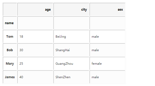
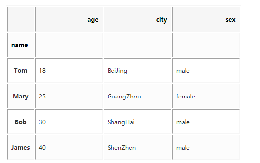
DataFrame 是一个带有索引的二维数据结构,每列可以有自己的名字,并且可以有不同的数据类型。你可以把它想象成一个 excel 表格或者数据库中的一张表,DataFrame 是最常用的 Pandas 对象。
  index = pd.Index(data=["Tom", "Bob", "Mary", "James"], name="name")

  data = {
      "age": [18, 30, 25, 40],
      "city": ["BeiJing", "ShangHai", "GuangZhou", "ShenZhen"]
  }

  user_info = pd.DataFrame(data=data, index=index)
  user_info

-
通过索引名来访问某行,这种办法需要借助 loc 方法
user_info.loc["Tom"] age 18 city BeiJing Name: Tom, dtype: object -
通过这行所在的位置来选择这一行
user_info.iloc[0] age 18 city BeiJing Name: Tom, dtype: object -
如何访问多行
user_info.iloc[1:3]

-
访问列
  user_info.age
  name
  Tom      18
  Bob      30
  Mary     25
  James    40
  Name: age, dtype: int64

  user_info["age"]
  name
  Tom      18
  Bob      30
  Mary     25
  James    40
  Name: age, dtype: int64

  #可以变换列的顺序
  user_info[["city", "age"]]
2.4 DataFrame数据处理操作
-
info 函数(类型和缺失值统计)
 user_info.info()

 Index: 4 entries, Tom to James
 Data columns (total 3 columns):
 age     4 non-null int64
 city    4 non-null object
 sex     4 non-null object
 dtypes: int64(1), object(2)
 memory usage: 128.0+ bytes

 user_info.head(2)

 user_info.shape
 (4, 3)

 user_info.T

-
通过 DataFrame 来获取它包含的原有数据
user_info.values array([[18, 'BeiJing', 'male'], [30, 'ShangHai', 'male'], [25, 'GuangZhou', 'female'], [40, 'ShenZhen', 'male']], dtype=object) -
统计
user_info.age.max() -
累加求和
user_info.age.cumsum() name Tom 18 Bob 48 Mary 73 James 113 Name: age, dtype: int64 user_info.sex.cumsum() name Tom male Bob malemale Mary malemalefemale James malemalefemalemale Name: sex, dtype: object -
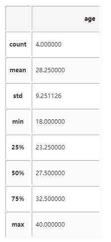
统计指标汇总(总数、平均数、标准差、最小值、最大值、25%/50%/75% 分位数)
user_info.describe()
user_info.describe(include=["object"])

-
统计下某列中每个值出现的次数
user_info.sex.value_counts() male 3 female 1 Name: sex, dtype: int64 -
获取某列最大值或最小值对应的索引
user_info.age.idxmax() 'James' -
离散化(分桶)
pd.cut(user_info.age, 3) name Tom (17.978, 25.333] Bob (25.333, 32.667] Mary (17.978, 25.333] James (32.667, 40.0] Name: age, dtype: category Categories (3, interval[float64]): [(17.978, 25.333] < (25.333, 32.667] < (32.667, 40.0]] -
自定义分桶
pd.cut(user_info.age, [1, 18, 30, 50]) name Tom (1, 18] Bob (18, 30] Mary (18, 30] James (30, 50] Name: age, dtype: category Categories (3, interval[int64]): [(1, 18] < (18, 30] < (30, 50]] -
离散化之后,给每个区间起个名字
pd.cut(user_info.age, [1, 18, 30, 50], labels=["childhood", "youth", "middle"]) name Tom childhood Bob youth Mary youth James middle Name: age, dtype: category Categories (3, object): [childhood < youth < middle] -
按照索引进行正序排的
user_info.sort_index()
-
按照列进行倒序排,可以设置参数 axis=1 和 ascending=False。
user_info.sort_index(axis=1, ascending=False) -
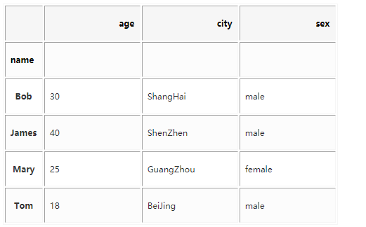
按照实际值来排序
user_info.sort_values(by="age")
user_info.sort_values(by=["age", "city"])
-
获取最大的n个值或最小值的n个值
user_info.age.nlargest(2) name James 40 Bob 30 Name: age, dtype: int64 -
函数应用map
user_info.age.map(lambda x: "yes" if x >= 30 else "no") name Tom no Bob yes Mary no James yes Name: age, dtype: object city_map = { "BeiJing": "north", "ShangHai": "south", "GuangZhou": "south", "ShenZhen": "south" } # 传入一个 map user_info.city.map(city_map) name Tom north Bob south Mary south James south Name: city, dtype: object -
函数应用apply
# 对 Series 来说,apply 方法 与 map 方法区别不大。 user_info.age.apply(lambda x: "yes" if x >= 30 else "no") name Tom no Bob yes Mary no James yes Name: age, dtype: object # 对 DataFrame 来说,apply 方法的作用对象是一行或一列数据(一个Series) user_info.apply(lambda x: x.max(), axis=0) age 40 city ShenZhen sex male dtype: object -
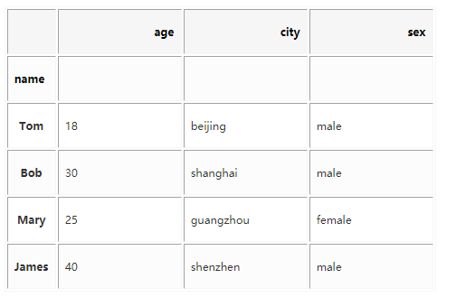
作用于 DataFrame 中的每个元素applymap
user_info.applymap(lambda x: str(x).lower())
-
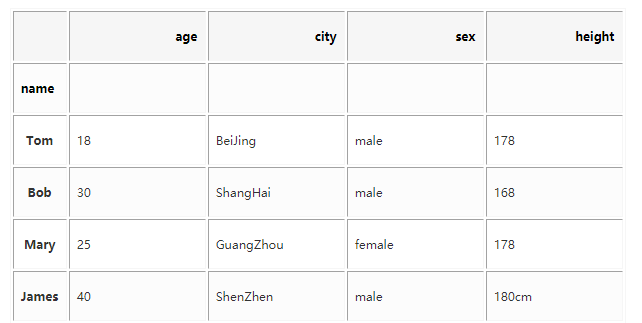
添加新列
  user_info["height"] = ["178", "168", "178", "180cm"]
  user_info
-
类型转换
  默认情况下,errors='raise',这意味着强转失败后直接抛出异常,设置 errors='coerce'
  可以在强转失败时将有问题的元素赋值为 pd.NaT(对于datetime和timedelta)或
  np.nan(数字)。设置 errors='ignore' 可以在强转失败时返回原有的数据。

  pd.to_numeric(user_info.height, errors="coerce")

  name
  Tom      178.0
  Bob      168.0
  Mary     178.0
  James      NaN
  Name: height, dtype: float64

  pd.to_numeric(user_info.height, errors="ignore")
  name
  Tom        178
  Bob        168
  Mary       178
  James    180cm
  Name: height, dtype: object
2.5 缺失值处理
待补充
2.6 Pandas案例实战
2.6.1 案例实战1
    import pandas
    food_info = pandas.read_csv("C:\\ML\\MLData\\food_info.csv")
    col_names = food_info.columns.tolist()
    print(col_names)
    print(food_info.head(3))

    针对某一列进行四则运算
    #print food_info["Iron_(mg)"]
    #div_1000 = food_info["Iron_(mg)"] / 1000
    #print div_1000
    # Adds 100 to each value in the column and returns a Series object.
    #add_100 = food_info["Iron_(mg)"] + 100

    # Subtracts 100 from each value in the column and returns a Series object.
    #sub_100 = food_info["Iron_(mg)"] - 100

    # Multiplies each value in the column by 2 and returns a Series object.
    #mult_2 = food_info["Iron_(mg)"]*2

    #It applies the arithmetic operator to the first value in both columns, the second value in both columns, and so on
    water_energy = food_info["Water_(g)"] * food_info["Energ_Kcal"]
    water_energy = food_info["Water_(g)"] * food_info["Energ_Kcal"]
    iron_grams = food_info["Iron_(mg)"] / 1000
    food_info["Iron_(g)"] = iron_grams

    #追加新列
    max_calories = food_info["Energ_Kcal"].max()
    print(max_calories)
    # Divide the values in "Energ_Kcal" by the largest value.
    normalized_calories = food_info["Energ_Kcal"] / max_calories
    normalized_protein = food_info["Protein_(g)"] / food_info["Protein_(g)"].max()
    normalized_fat = food_info["Lipid_Tot_(g)"] / food_info["Lipid_Tot_(g)"].max()
    food_info["Normalized_Protein"] = normalized_protein
    food_info["Normalized_Fat"] = normalized_fat

    #排序
    #By default, pandas will sort the data by the column we specify in ascending order and return a new DataFrame
    # Sorts the DataFrame in-place, rather than returning a new DataFrame.
    #print food_info["Sodium_(mg)"]
    food_info.sort_values("Sodium_(mg)", inplace=True)
    #print (food_info["Sodium_(mg)"])
    #Sorts by descending order, rather than ascending.
    food_info.sort_values("Sodium_(mg)", inplace=True, ascending=False)
    print (food_info["Sodium_(mg)"])

2.6.2 泰坦尼克案例实战2
import pandas as pd
import numpy as np
titanic_survival = pd.read_csv("C:\\ML\\MLData\\titanic_train.csv")
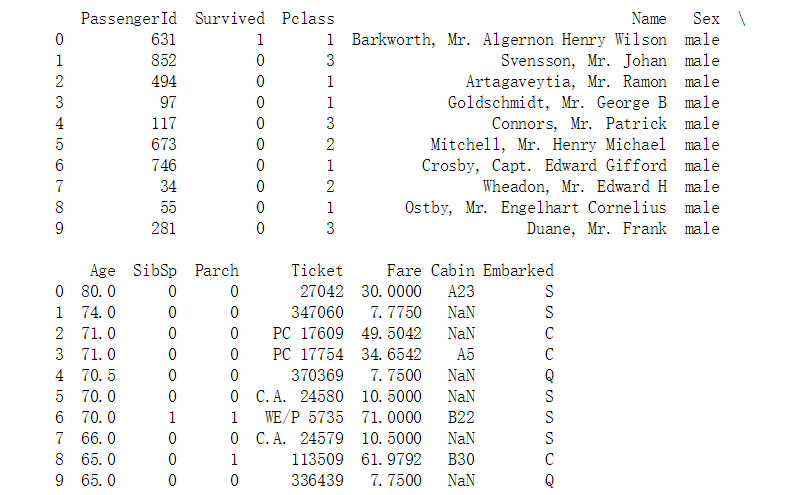
#SibSp:老人和孩子
#Parch:家人
#Pclass:仓位级别
#Cabin:船舱编号,NaN是缺失值(就是为空的值)
#Embarked 登船地点 S C Q 三个码头
titanic_survival.head()

-
控制空值判断及展示
#The Pandas library uses NaN, which stands for "not a number", to indicate a missing value. #we can use the pandas.isnull() function which takes a pandas series and returns a series of True and False values age = titanic_survival["Age"] #print(age.loc[0:10]) age_is_null = pd.isnull(age) #print (age_is_null) age_null_true = age[age_is_null] print (age_null_true) age_null_count = len(age_null_true) #print(age_null_count) 5 NaN 17 NaN 19 NaN 26 NaN 28 NaN 29 NaN 31 NaN 32 NaN 36 NaN 42 NaN 45 NaN 46 NaN -
含有空值时将无法计算
#The result of this is that mean_age would be nan. This is because any calculations we do with a null value also result in a null value mean_age = sum(titanic_survival["Age"]) / len(titanic_survival["Age"]) print (mean_age) nan #过滤出非空值,但是略显复杂 #we have to filter out the missing values before we calculate the mean. good_ages = titanic_survival["Age"][age_is_null == False] #print good_ages correct_mean_age = sum(good_ages) / len(good_ages) print (correct_mean_age) 29.69911764705882 # missing data is so common that many pandas methods automatically filter for it correct_mean_age = titanic_survival["Age"].mean() print correct_mean_age 29.6991176471 #mean fare for each class -
每个船舱位的平均价格
passenger_classes = [1, 2, 3] fares_by_class = {} for this_class in passenger_classes: pclass_rows = titanic_survival[titanic_survival["Pclass"] == this_class] pclass_fares = pclass_rows["Fare"] fare_for_class = pclass_fares.mean() fares_by_class[this_class] = fare_for_class print (fares_by_class) {1: 84.15468749999992, 2: 20.66218315217391, 3: 13.675550101832997} # pandas不同列之间的关系,pivot_table高级用法 passenger_survival = titanic_survival.pivot_table(index="Pclass", values="Survived", aggfunc=np.mean) print (passenger_survival) Survived Pclass 1 0.629630 2 0.472826 3 0.242363 # 默认求均值 passenger_age = titanic_survival.pivot_table(index="Pclass", values="Age") print(passenger_age) Pclass 1 38.233441 2 29.877630 3 25.140620 Name: Age, dtype: float64 #多列之间关系 port_stats = titanic_survival.pivot_table(index="Embarked", values=["Fare","Survived"], aggfunc=np.sum) print(port_stats) Fare Survived Embarked C 10072.2962 93 Q 1022.2543 30 S 17439.3988 217 -
丢掉缺失值 axis=1 表示行
#specifying axis=1 or axis='columns' will drop any columns that have null values drop_na_columns = titanic_survival.dropna(axis=1) new_titanic_survival = titanic_survival.dropna(axis=0,subset=["Age", "Sex"]) #print new_titanic_survival -
通过索引和列名
row_index_83_age = titanic_survival.loc[83,"Age"] row_index_1000_pclass = titanic_survival.loc[766,"Pclass"] print (row_index_83_age) print (row_index_1000_pclass) 28.0 1 -
按值排序(索引不变),并重设索引
  #按值排序(索引不变)
  new_titanic_survival = titanic_survival.sort_values("Age",ascending=False)
  #print (new_titanic_survival[0:10])

  #索引发生变化
  itanic_reindexed = new_titanic_survival.reset_index(drop=True)
  print(itanic_reindexed.iloc[0:10])
-
返回第100行数据
# This function returns the hundredth item from a series def hundredth_row(column): # Extract the hundredth item hundredth_item = column.iloc[99] return hundredth_item # Return the hundredth item from each column hundredth_row = titanic_survival.apply(hundredth_row) print (hundredth_row) PassengerId 100 Survived 0 Pclass 2 Name Kantor, Mr. Sinai Sex male Age 34 SibSp 1 Parch 0 Ticket 244367 Fare 26 Cabin NaN Embarked S dtype: object -
自定义行数非空判断
def not_null_count(column): column_null = pd.isnull(column) null = column[column_null] return len(null) column_null_count = titanic_survival.apply(not_null_count) print (column_null_count) PassengerId 0 Survived 0 Pclass 0 Name 0 Sex 0 Age 177 SibSp 0 Parch 0 Ticket 0 Fare 0 Cabin 687 Embarked 2 dtype: int64 -
定义级别axis=1表示行
#By passing in the axis=1 argument, we can use the DataFrame.apply() method to iterate over rows instead of columns. def which_class(row): pclass = row['Pclass'] if pd.isnull(pclass): return "Unknown" elif pclass == 1: return "First Class" elif pclass == 2: return "Second Class" elif pclass == 3: return "Third Class" classes = titanic_survival.apply(which_class, axis=1) print (classes) 0 Third Class 1 First Class 2 Third Class 3 First Class 4 Third Class 5 Third Class 6 First Class 7 Third Class -
自定义函数
def is_minor(row): if row["Age"] < 18: return True else: return False minors = titanic_survival.apply(is_minor, axis=1) #print minors def generate_age_label(row): age = row["Age"] if pd.isnull(age): return "unknown" elif age < 18: return "minor" else: return "adult" age_labels = titanic_survival.apply(generate_age_label, axis=1) print age_labels 0 adult 1 adult 2 adult 3 adult 4 adult 5 unknown 6 adult 7 minor 8 adult 9 minor 10 minor 11 adult 12 adult -
分类类别
 titanic_survival['age_labels'] = age_labels
 age_group_survival = titanic_survival.pivot_table(index="age_labels", values="Survived")
 print age_group_survival

 age_labels
 adult      0.381032
 minor      0.539823
 unknown    0.293785
 Name: Survived, dtype: float64
2.6.3 Series 案例实战3
    #Pandas默认其中一行或一列就是Series
    import pandas as pds
    fandango = pd.read_csv('C:\\ML\\MLData\\fandango_score_comparison.csv')
    series_film = fandango['FILM']
    print(series_film[0:5])
    series_rt = fandango['RottenTomatoes']
    print (series_rt[0:5])

    0    Avengers: Age of Ultron (2015)
    1                 Cinderella (2015)
    2                    Ant-Man (2015)
    3            Do You Believe? (2015)
    4     Hot Tub Time Machine 2 (2015)
    Name: FILM, dtype: object
    0    74
    1    85
    2    80
    3    18
    4    14
    Name: RottenTomatoes, dtype: int64
-
设置索引列,根据索引取得对应的值
# Import the Series object from pandas from pandas import Series film_names = series_film.values #print (type(film_names)) #print (film_names) rt_scores = series_rt.values #print (rt_scores) series_custom = Series(rt_scores , index=film_names) #根据索引取得对应的值 series_custom[['Minions (2015)', 'Leviathan (2014)']] Minions (2015) 54 Leviathan (2014) 99 dtype: int64 -
范围查找
series_custom = Series(rt_scores , index=film_names) #series_custom[['Minions (2015)', 'Leviathan (2014)']] fiveten = series_custom[5:10] print(fiveten) The Water Diviner (2015) 63 Irrational Man (2015) 42 Top Five (2014) 86 Shaun the Sheep Movie (2015) 99 Love & Mercy (2015) 89 dtype: int64 -
索引排序,并重设
original_index = series_custom.index.tolist() #print original_index sorted_index = sorted(original_index) sorted_by_index = series_custom.reindex(sorted_index) #print sorted_by_index '71 (2015) 97 5 Flights Up (2015) 52 A Little Chaos (2015) 40 A Most Violent Year (2014) 90 About Elly (2015) 97 Aloha (2015) 19 American Sniper (2015) 72 -
Series 值排序
sc2 = series_custom.sort_index() sc3 = series_custom.sort_values() #print(sc2[0:10]) print(sc3[0:10]) Paul Blart: Mall Cop 2 (2015) 5 Hitman: Agent 47 (2015) 7 Hot Pursuit (2015) 8 Fantastic Four (2015) 9 Taken 3 (2015) 9 The Boy Next Door (2015) 10 The Loft (2015) 11 Unfinished Business (2015) 11 Mortdecai (2015) 12 Seventh Son (2015) 12 -
Series对应索引相加
#The values in a Series object are treated as an ndarray, the core data type in NumPy import numpy as np # Add each value with each other print np.add(series_custom, series_custom) # Apply sine function to each value np.sin(series_custom) # Return the highest value (will return a single value not a Series) np.max(series_custom) -
Series对应Lambda表达式(求标准差)
#The apply() method in Pandas allows us to specify Python logic #The apply() method requires you to pass in a vectorized operation #that can be applied over each Series object. import numpy as np # returns the data types as a Series types = fandango_films.dtypes #print types # filter data types to just floats, index attributes returns just column names float_columns = types[types.values == 'float64'].index # use bracket notation to filter columns to just float columns float_df = fandango_films[float_columns] #print float_df # `x` is a Series object representing a column deviations = float_df.apply(lambda x: np.std(x)) print(deviations) Metacritic_User 1.505529 IMDB 0.955447 Fandango_Stars 0.538532 Fandango_Ratingvalue 0.501106 RT_norm 1.503265 RT_user_norm 0.997787 Metacritic_norm 0.972522 Metacritic_user_nom 0.752765 IMDB_norm 0.477723 -
对应两列通过Lambda表达式求标准差
  rt_mt_user = float_df[['RT_user_norm', 'Metacritic_user_nom']]
  rt_mt_user.apply(lambda x: np.std(x), axis=1)

  FILM
  Avengers: Age of Ultron (2015)                    0.375
  Cinderella (2015)                                 0.125
  Ant-Man (2015)                                    0.225
  Do You Believe? (2015)                            0.925
  Hot Tub Time Machine 2 (2015)                     0.150
  The Water Diviner (2015)                          0.150
  Irrational Man (2015)                             0.575
  Top Five (2014)                                   0.100
  Shaun the Sheep Movie (2015)                      0.150
  Love & Mercy (2015)                               0.050
  Far From The Madding Crowd (2015)                 0.050
  Black Sea (2015)                                  0.150
3 matplotlib使用实践

-
折线图
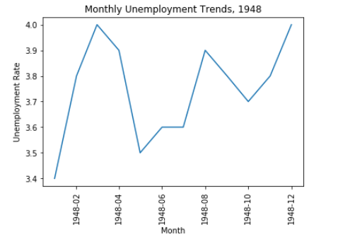
  import pandas as pd
  unrate = pd.read_csv("C:\\ML\\MLData\\unrate.csv")
  unrate['DATE'] = pd.to_datetime(unrate['DATE'])
  print(unrate.head(12))

        DATE      VALUE
  0  1948-01-01    3.4
  1  1948-02-01    3.8
  2  1948-03-01    4.0
  3  1948-04-01    3.9
  4  1948-05-01    3.5
  5  1948-06-01    3.6
  6  1948-07-01    3.6
  7  1948-08-01    3.9
  8  1948-09-01    3.8
  9  1948-10-01    3.7
  10 1948-11-01    3.8
  11 1948-12-01    4.0

  import matplotlib.pyplot as plt
  plt.plot()
  plt.show()
    first_twelve = unrate[0:12]
    plt.plot(first_twelve['DATE'], first_twelve['VALUE'])
    plt.show()
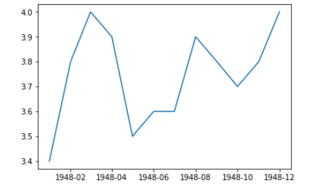
    plt.plot(first_twelve['DATE'], first_twelve['VALUE'])
    plt.xticks(rotation=45)
    #print help(plt.xticks)
    plt.show()
#xlabel(): accepts a string value, which gets set as the x-axis label.
#ylabel(): accepts a string value, which is set as the y-axis label.
#title(): accepts a string value, which is set as the plot title.

plt.plot(first_twelve['DATE'], first_twelve['VALUE'])
plt.xticks(rotation=90)
plt.xlabel('Month')
plt.ylabel('Unemployment Rate')
plt.title('Monthly Unemployment Trends, 1948')
plt.show()
-
多条折线图展示
  fig = plt.figure(figsize=(10,6))
  colors = ['red', 'blue', 'green', 'orange', 'black']
  for i in range(5):
      start_index = i*12
      end_index = (i+1)*12
      subset = unrate[start_index:end_index]
      label = str(1948 + i)
      plt.plot(subset['MONTH'], subset['VALUE'], c=colors[i], label=label)
  plt.legend(loc='upper left')
  plt.xlabel('Month, Integer')
  plt.ylabel('Unemployment Rate, Percent')
  plt.title('Monthly Unemployment Trends, 1948-1952')

  plt.show()

-
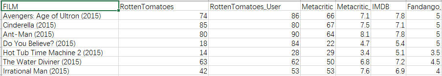
柱状图竖型展示
  import pandas as pd
  reviews = pd.read_csv('C:\\ML\\MLData\\fandango_scores.csv')
  cols = ['FILM', 'RT_user_norm', 'Metacritic_user_nom', 'IMDB_norm', 'Fandango_Ratingvalue', 'Fandango_Stars']
  norm_reviews = reviews[cols]
  print(type(reviews))
  #打印出第一行
  print(norm_reviews[:1])

  <class 'pandas.core.frame.DataFrame'>

    import matplotlib.pyplot as plt
    from numpy import arange

    #取出第一行指定列num_cols的数据
    num_cols = ['RT_user_norm', 'Metacritic_user_nom', 'IMDB_norm', 'Fandango_Ratingvalue', 'Fandango_Stars']
    bar_heights = norm_reviews.loc[0, num_cols].values
    print(bar_heights)

    [4.3 3.55 3.9 4.5 5.0]

    bar_heights = norm_reviews.loc[0, num_cols].values
    #横轴位置
    bar_positions = arange(5) + 0.75
    #横轴标识的位置(1到6之间)
    tick_positions = range(1,6)

    fig, ax = plt.subplots()
    #0.5标识柱状图宽度
    ax.bar(bar_positions, bar_heights, 0.5)
    ax.set_xticks(tick_positions)
    ax.set_xticklabels(num_cols, rotation=90)

    ax.set_xlabel('Rating Source')
    ax.set_ylabel('Average Rating')
    ax.set_title('Average User Rating For Avengers: Age of Ultron (2015)')
    plt.show()

-
柱状图横向表示
  import matplotlib.pyplot as plt
  from numpy import arange
  num_cols = ['RT_user_norm', 'Metacritic_user_nom', 'IMDB_norm', 'Fandango_Ratingvalue', 'Fandango_Stars']

  bar_widths = norm_reviews.loc[0, num_cols].values
  bar_positions = arange(5) + 0.75
   #横轴标识名的位置(1到6之间)
  tick_positions = range(1,6)
  fig, ax = plt.subplots()
  ax.barh(bar_positions, bar_widths, 0.6)

  ax.set_yticks(tick_positions)
  ax.set_yticklabels(num_cols)
  ax.set_ylabel('Rating Source')
  ax.set_xlabel('Average Rating')
  ax.set_title('Average User Rating For Avengers: Age of Ultron (2015)')
  plt.show()

-
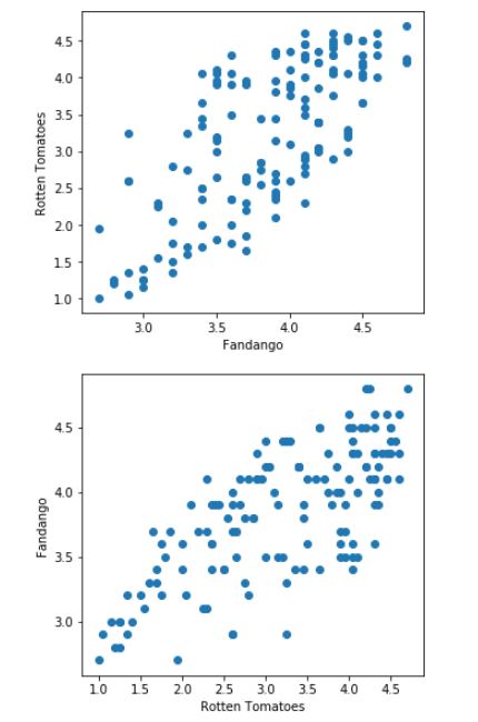
散点图
  #Switching Axes
  fig = plt.figure(figsize=(5,10))
  ax1 = fig.add_subplot(2,1,1)
  ax2 = fig.add_subplot(2,1,2)
  ax1.scatter(norm_reviews['Fandango_Ratingvalue'], norm_reviews['RT_user_norm'])
  ax1.set_xlabel('Fandango')
  ax1.set_ylabel('Rotten Tomatoes')
  ax2.scatter(norm_reviews['RT_user_norm'], norm_reviews['Fandango_Ratingvalue'])
  ax2.set_xlabel('Rotten Tomatoes')
  ax2.set_ylabel('Fandango')
  plt.show()
- Hist的bins区间统计
import pandas as pd
import matplotlib.pyplot as plt
reviews = pd.read_csv('C:\\ML\\MLData\\fandango_scores.csv')
cols = ['FILM', 'RT_user_norm', 'Metacritic_user_nom', 'IMDB_norm', 'Fandango_Ratingvalue']
norm_reviews = reviews[cols]
print(norm_reviews[:5])
#按照列进行分组聚合
fandango_distribution = norm_reviews['Fandango_Ratingvalue'].value_counts()
fandango_distribution = fandango_distribution.sort_index()
#按照列进行分组聚合
imdb_distribution = norm_reviews['IMDB_norm'].value_counts()
imdb_distribution = imdb_distribution.sort_index()
print(fandango_distribution)
2.7 2
2.8 2
2.9 5
3.0 4
3.1 3
3.2 5
3.3 4
3.4 9
3.5 9
3.6 8
3.7 9
3.8 5
3.9 12
4.0 7
4.1 16
4.2 12
4.3 11
4.4 7
4.5 9
4.6 4
4.8 3
Name: Fandango_Ratingvalue, dtype: int64
print(imdb_distribution)
2.00 1
2.10 1
2.15 1
2.20 1
2.30 2
2.45 2
2.50 1
2.55 1
2.60 2
2.70 4
2.75 5
2.80 2
2.85 1
2.90 1
2.95 3
3.00 2
3.05 4
3.10 1
3.15 9
3.20 6
3.25 4
3.30 9
3.35 7
3.40 1
3.45 7
3.50 4
3.55 7
3.60 10
3.65 5
3.70 8
3.75 6
3.80 3
3.85 4
3.90 9
3.95 2
4.00 1
4.05 1
4.10 4
4.15 1
4.20 2
4.30 1
Name: IMDB_norm, dtype: int64
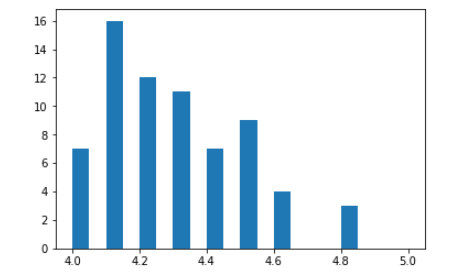
fig, ax = plt.subplots()
#ax.hist(norm_reviews['Fandango_Ratingvalue'])
#ax.hist(norm_reviews['Fandango_Ratingvalue'],bins=20)
指定区间为20个,范围为4到5
ax.hist(norm_reviews['Fandango_Ratingvalue'], range=(4, 5),bins=20)
plt.show()
-
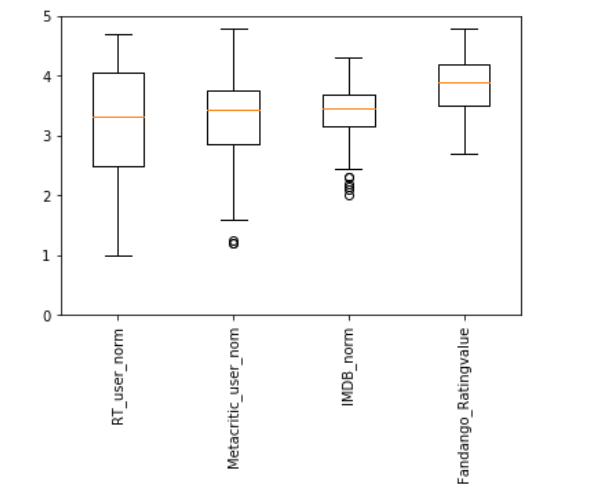
4分图盒图
  num_cols = ['RT_user_norm', 'Metacritic_user_nom', 'IMDB_norm', 'Fandango_Ratingvalue']
  fig, ax = plt.subplots()
  #指定统计列取出对应值
  ax.boxplot(norm_reviews[num_cols].values)
  ax.set_xticklabels(num_cols, rotation=90)
  ax.set_ylim(0,5)
  plt.show()
4 Seaborn专业可视化库(基于matplot)
-
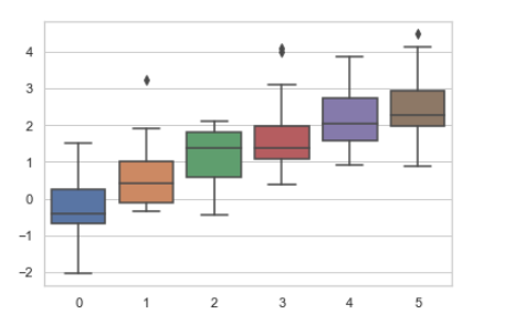
风格设置
  import seaborn as sns
  import numpy as np
  import matplotlib as mpl
  import matplotlib.pyplot as plt
  %matplotlib inline

  sns.set_style("whitegrid")
  data = np.random.normal(size=(20, 6)) + np.arange(6) / 2
  sns.boxplot(data=data)
     sns.set_style("dark")
     sinplot()

    sns.set_style("white")
    sinplot()

    sns.set_style("whitegrid")
    sns.boxplot(data=data, palette="deep")
    sns.despine(left=True)
-
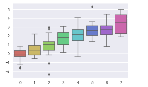
调色板设置
  import numpy as np
  import seaborn as sns
  import matplotlib.pyplot as plt
  %matplotlib inline
  sns.set(rc={"figure.figsize": (6, 6)})

  current_palette = sns.color_palette()
  sns.palplot(current_palette)

    6个默认的颜色循环主题: deep, muted, pastel, bright, dark, colorblind

    sns.palplot(sns.color_palette("hls", 8))

    data = np.random.normal(size=(20, 8)) + np.arange(8) / 2
    sns.boxplot(data=data,palette=sns.color_palette("hls", 8))

    data = np.random.normal(size=(20, 8)) + np.arange(8) / 2
    #print(data)
    sns.boxplot(data=data,palette=sns.color_palette("hls", 8))
-
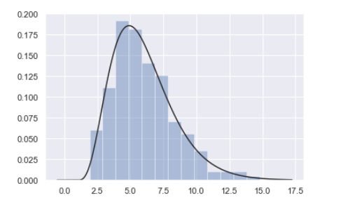
区间直方图绘制(kde是否指定核密度估计)
  x = np.random.gamma(6, size=200)
  sns.distplot(x, kde=False, fit=stats.gamma)
-
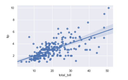
线性回归1
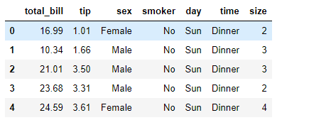
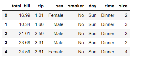
  %matplotlib inline
  import numpy as np
  import pandas as pd
  import matplotlib as mpl
  import matplotlib.pyplot as plt

  import seaborn as sns
  sns.set(color_codes=True)
  np.random.seed(sum(map(ord, "regression")))
  tips = sns.load_dataset("tips")
  tips.head()
sns.regplot(x="total_bill", y="tip", data=tips)
-
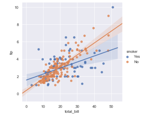
线性回归2
sns.lmplot(x="total_bill", y="tip", hue="smoker", data=tips);
-
多分类问题
  %matplotlib inline
  import numpy as np
  import pandas as pd
  import matplotlib as mpl
  import matplotlib.pyplot as plt
  import seaborn as sns
  sns.set(style="whitegrid", color_codes=True)

  np.random.seed(sum(map(ord, "categorical")))
  titanic = sns.load_dataset("titanic")
  tips = sns.load_dataset("tips")
  iris = sns.load_dataset("iris")
  sns.stripplot(x="day", y="total_bill", data=tips);
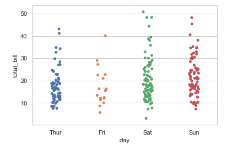
sns.stripplot(x="day", y="total_bill", data=tips, jitter=True)
-
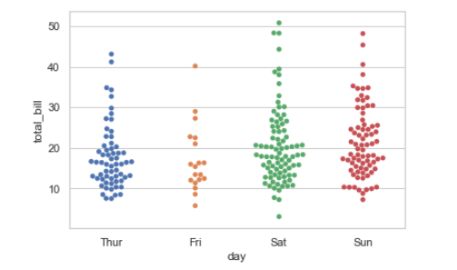
树桩展示均匀展示
sns.swarmplot(x="day", y="total_bill", data=tips)
-
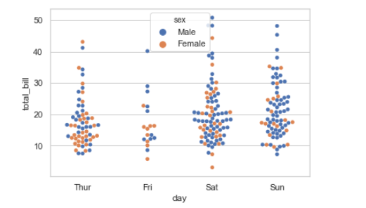
树桩展示均匀并分类展示
sns.swarmplot(x="day", y="total_bill", hue="sex",data=tips)
-
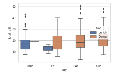
盒图
 IQR即统计学概念四分位距,第一/四分位与第三/四分位之间的距离
 N = 1.5IQR 如果一个值>Q3+N或 < Q1-N,则为离群点

 #横杠最小值和最大值
 sns.boxplot(x="day", y="total_bill", hue="time", data=tips);
-
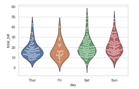
小提琴图(越胖包含的数据越多)
sns.violinplot(x="day", y="total_bill", hue="sex", data=tips, split=True); -
葫芦图
 sns.violinplot(x="day", y="total_bill", data=tips, inner=None)
 sns.swarmplot(x="day", y="total_bill", data=tips, color="w", alpha=.5)

-
柱状分类统计图
sns.barplot(x="sex", y="survived", hue="class", data=titanic);

-
点图可以更好的描述变化差异
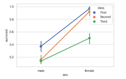
sns.pointplot(x="sex", y="survived", hue="class", data=titanic);
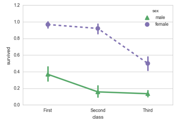
    sns.pointplot(x="class", y="survived", hue="sex", data=titanic,
          palette={"male": "g", "female": "m"},
          markers=["^", "o"], linestyles=["-", "--"]);
-
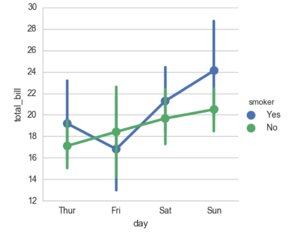
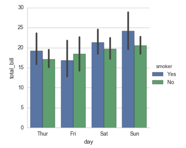
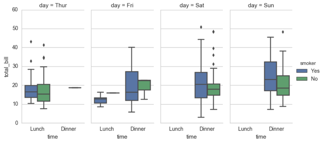
多层面板分类图
sns.factorplot(x="day", y="total_bill", hue="smoker", data=tips)
sns.factorplot(x="day", y="total_bill", hue="smoker", data=tips, kind="bar")
    sns.factorplot(x="day", y="total_bill", hue="smoker",
              col="time", data=tips, kind="swarm")
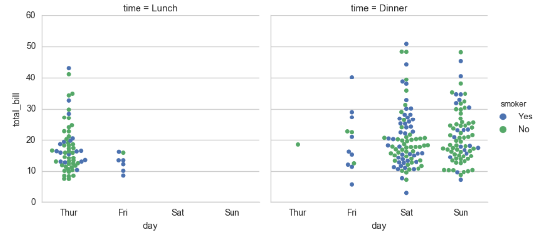
    sns.factorplot(x="time", y="total_bill", hue="smoker",
           col="day", data=tips, kind="box", size=4, aspect=.5)
-
FacetGrid 多参数网格面板
  %matplotlib inline
  import numpy as np
  import pandas as pd
  import seaborn as sns
  from scipy import stats
  import matplotlib as mpl
  import matplotlib.pyplot as plt

  sns.set(style="ticks")
  np.random.seed(sum(map(ord, "axis_grids")))
  tips = sns.load_dataset("tips")
  tips.head()
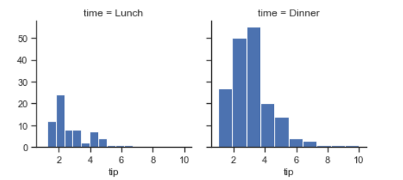
    g = sns.FacetGrid(tips, col="time")
    g.map(plt.hist, "tip");
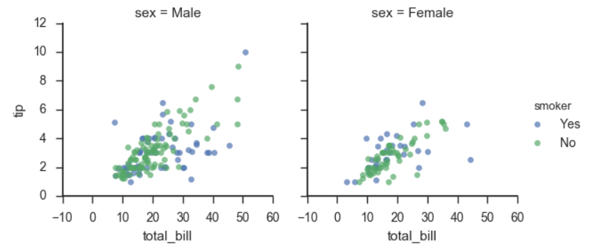
    g = sns.FacetGrid(tips, col="sex", hue="smoker")
    g.map(plt.scatter, "total_bill", "tip", alpha=.7)
    g.add_legend();
    g = sns.FacetGrid(tips, row="smoker", col="time", margin_titles=True)
    g.map(sns.regplot, "size", "total_bill", color=".1", fit_reg=False, x_jitter=.1);

-
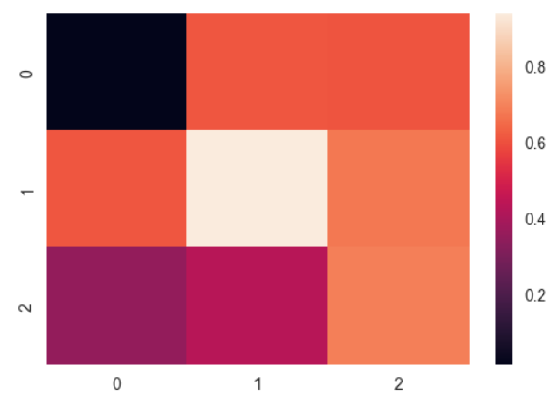
热力图
   %matplotlib inline
  import matplotlib.pyplot as plt
  import numpy as np;
  np.random.seed(0)
  import seaborn as sns;
  sns.set()
  uniform_data = np.random.rand(3, 3)
  print (uniform_data)
  heatmap = sns.heatmap(uniform_data)

  [[ 0.0187898   0.6176355   0.61209572]
   [ 0.616934    0.94374808  0.6818203 ]
   [ 0.3595079   0.43703195  0.6976312 ]]
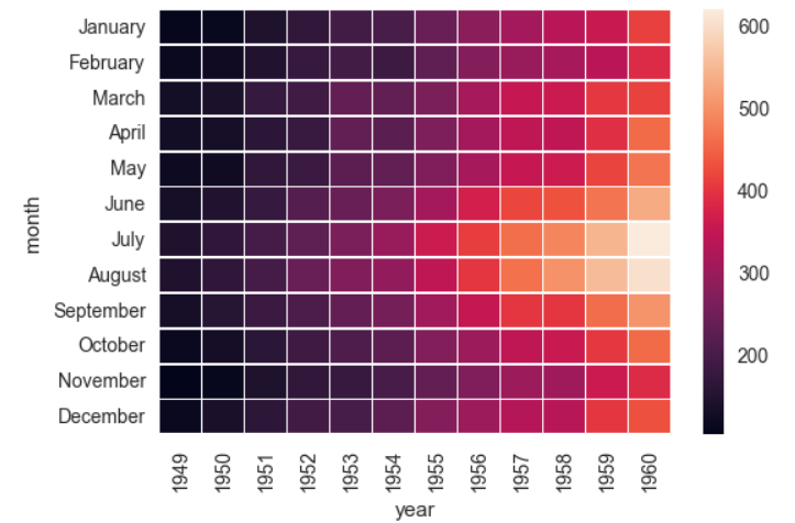
ax = sns.heatmap(flights, linewidths=.5)
5 总结
方便复习,整成笔记,内容粗略,勿怪,待完善。
版权声明:本套技术专栏是作者(秦凯新)平时工作的总结和升华,通过从真实商业环境抽取案例进行总结和分享,并给出商业应用的调优建议和集群环境容量规划等内容,请持续关注本套博客。QQ邮箱地址:1120746959@qq.com,如有任何学术交流,可随时联系。
秦凯新 于深圳
。


 6593
6593


 被折叠的 条评论
为什么被折叠?
被折叠的 条评论
为什么被折叠?
 到【灌水乐园】发言


