


多变量线性回归
在这一部分中,您将实现具有多个变量的线性回归
预测房屋价格。 假设你要卖掉你的房子,而你
想知道好的市场价格是多少。 一种方法是
首先收集最近出售的房屋信息并制作房屋模型
价格。
文件 ex1data2.txt 包含 Port- 的房价训练集
土地,俄勒冈州。 第一列是房子的大小(以平方英尺为单位),
第二列是卧室数量,第三列是价格
在这所房子里面。
ex1 multi.m 脚本已设置为帮助您逐步完成此操作
锻炼
特征归一化
ex1 multi.m 脚本将首先加载和显示一些值
从这个数据集中。通过查看这些值,请注意房屋大小约为
卧室数量的1000倍。当特征按 mag- 顺序不同时
nitude,首先执行特征缩放可以使梯度下降收敛
快得多。
您在这里的任务是完成 featureNormalize.m 中的代码以
• 从数据集中减去每个特征的平均值。
• 减去平均值后,额外缩放(除)特征值
通过它们各自的“标准偏差”。
import numpy as np
import pandas as pd
import matplotlib.pyplot as plt
# 代价函数
def computeCost(X, Y, theta):
inner = np.power((X * theta.T) - Y, 2)
return np.sum(inner) / (2 * len(X))
# 梯度下降假设函数和批量梯度下降更新规则不变。
def gradientDescent(X, Y, theta, alpha, iters):
temp = np.matrix(np.zeros(theta.shape))
parameters = int(theta.shape[1])
cost = np.zeros(iters)
for i in range(iters):
error = X * theta.T - Y
for j in range(parameters):
term = np.multiply(error, X[:, j])
temp[0, j] = temp[0, j] - alpha / len(X) * np.sum(term)
theta = temp
cost[i] = computeCost(X, Y, theta)
return theta, cost
path = 'ex1data2.txt'
data = pd.read_csv(path, header=None, names=['Size', 'Bedrooms', 'Price'])
data.head()
# 保存mean、std、mins、maxs、data
means = data.mean().values
stds = data.std().values
mins = data.min().values
maxs = data.max().values
data_ = data.values
data.describe()
# 特征缩放
data = (data - data.mean()) / data.std()
data.head()
# add ones column
data.insert(0, 'Ones', 1)
# set X (training data) and Y (target variable)
cols = data.shape[1]
X = data.iloc[:, :cols-1]
Y = data.iloc[:, cols-1:cols]
# convert to matrices and initialize theta
X = np.matrix(X.values)
Y = np.matrix(Y.values)
theta = np.matrix(np.array([0, 0, 0]))
# perform linear regression on the data set
alpha = 0.01
iters = 1000
g, cost = gradientDescent(X, Y, theta, alpha, iters)
# get the cost(error) of the model
computeCost(X, Y, g)
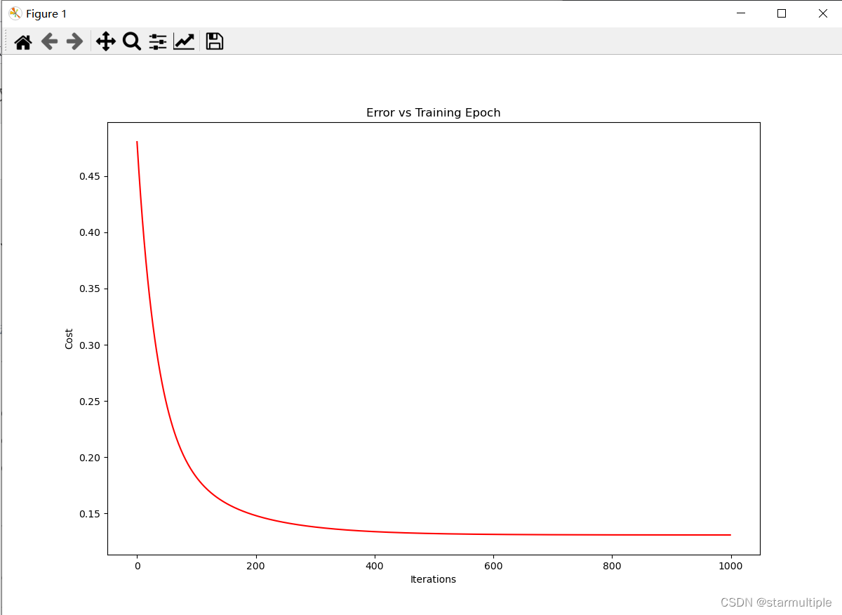
# 画出cost图像
fig, ax = plt.subplots(figsize=(12, 8))
ax.plot(np.arange(iters), cost, 'r')
ax.set_xlabel('Iterations')
ax.set_ylabel('Cost')
ax.set_title('Error vs Training Epoch')
plt.show()
#参数转化为缩放前
def theta_transform(theta, means, stds):
temp = means[:-1] * theta[1:] / stds[:-1]
theta[0] = (theta[0] - np.sum(temp)) * stds[-1] + means[-1]
theta[1:] = theta[1:] * stds[-1] / stds[:-1]
return theta.reshape(1, -1)
g_ = np.array(g.reshape(-1, 1))
means = means.reshape(-1, 1)
stds = stds.reshape(-1, 1)
transform_g = theta_transform(g_, means, stds)
transform_g
# 预测价格
def predictPrice(x, y, theta):
return theta[0, 0] + theta[0, 1]*x + theta[0, 2]*y
# 2104,3,399900,
price = predictPrice(2104, 3, transform_g)
price
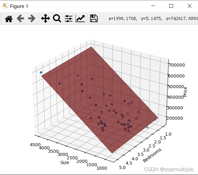
# 画出拟合平面
from mpl_toolkits.mplot3d import Axes3D
fig = plt.figure()
ax = Axes3D(fig)
X_ = np.arange(mins[0], maxs[0]+1, 1)
Y_ = np.arange(mins[1], maxs[1]+1, 1)
X_, Y_ = np.meshgrid(X_, Y_)
Z_ = transform_g[0,0] + transform_g[0,1] * X_ + transform_g[0,2] * Y_
# 手动设置角度
ax.view_init(elev=25, azim=125)
ax.set_xlabel('Size')
ax.set_ylabel('Bedrooms')
ax.set_zlabel('Price')
ax.plot_surface(X_, Y_, Z_, rstride=1, cstride=1, color='red')
ax.scatter(data_[:, 0], data_[:, 1], data_[:, 2])
plt.show()
# print(data2_, data2_.shape, type(data2_))


 113
113


 被折叠的 条评论
为什么被折叠?
被折叠的 条评论
为什么被折叠?
 到【灌水乐园】发言


