


实验环境
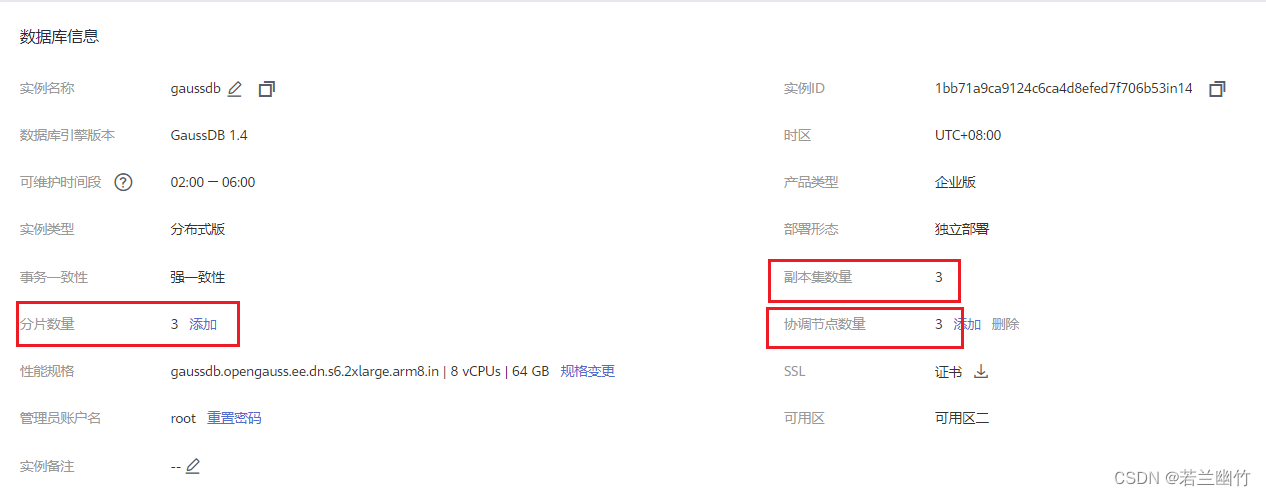
- 华为云GaussDB云数据库,规则如下:
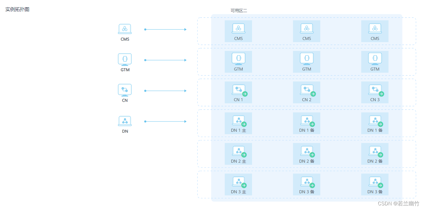
- 集群拓扑结构,如下:
一、分布式架构
-
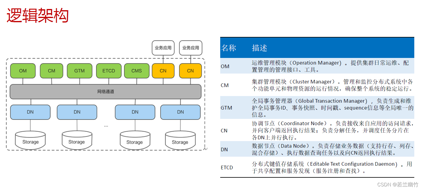
逻辑架构
-
常用部署方式
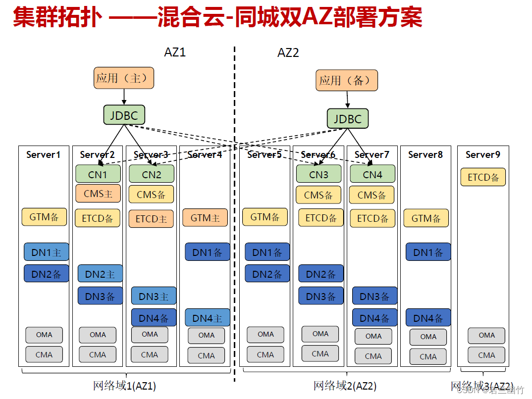
部署说明:
1.双AZ采用带第三方仲裁方式部署,即独立Server9网络域
2.4C4D4副本,一共需要9台物理机(4+4+1)
3.DN主备交叉部署,主统一在AZ1
4.主机故障优先在同AZ切换
5.核心组件两个AZ对称,支持跨AZ双活;
二、分片和分区
-
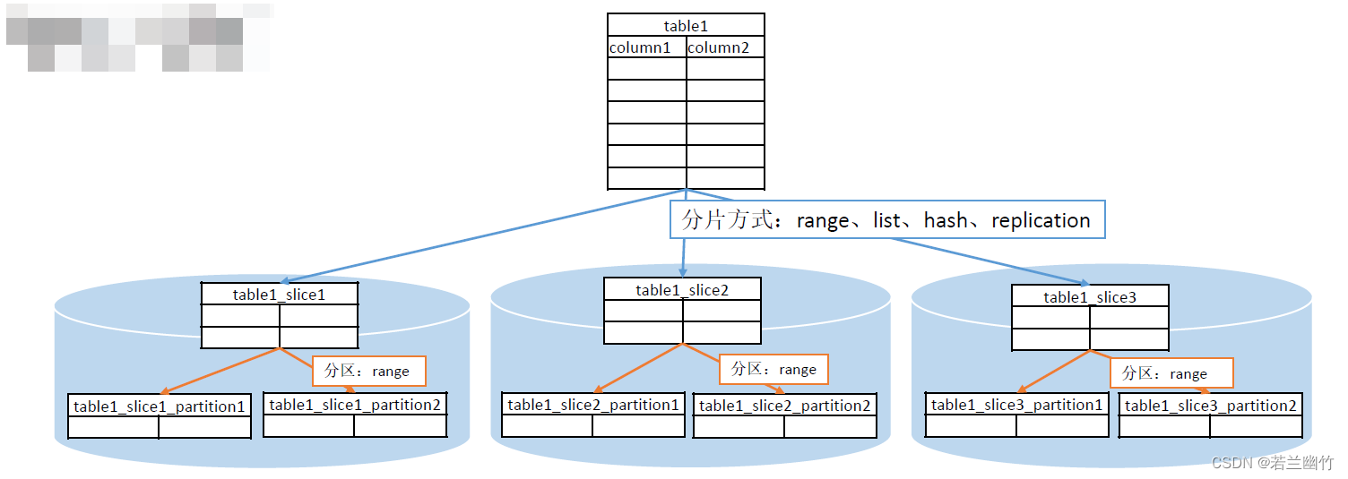
分片:
- REPLICATION:表的每一行存在所有数据节点(DN)中,即每个数据节点都有完整的表数据。
- HASH:对指定的列进行Hash,通过映射,把数据分布到指定DN。
- RANGE:对指定列按照范围进行映射,把数据分布到对应DN。
- LIST :对指定列按照具体值进行映射,把数据分布到对应DN。
-
分区:
如RANGE:类似二级分区,单机上的分区功能 -
两者关系:
-
数据分片示例
- 查询节点名称
结果如下:SELECT * FROM pgxc_node where node_type='D';postgres=> SELECT * FROM pgxc_node where node_type='D'; node_name | node_type | node_port | node_host | node_port1 | node_host1 | hostis_primary | nodeis_primary | nodeis_preferred | node_id | sctp_port | control_port | sctp_port1 | control_port1 | nodeis_central | nodeis_active -------------------+-----------+-----------+---------------+------------+---------------+----------------+----------------+------------------+-------------+-----------+--------------+------------+---------------+----------------+--------------- dn_6001_6002_6003 | D | 40000 | 192.168.0.230 | 40000 | 192.168.0.230 | t | f | f | -1072999043 | 40002 | 40003 | 0 | 0 | f | t dn_6004_6005_6006 | D | 40000 | 192.168.0.193 | 40000 | 192.168.0.193 | t | f | f | -564789568 | 40002 | 40003 | 0 | 0 | f | t dn_6007_6008_6009 | D | 40000 | 192.168.0.122 | 40000 | 192.168.0.122 | t | f | f | 1532339558 | 40002 | 40003 | 0 | 0 | f | t (3 rows) - 创建组
create node group group_dn1_dn2 with(dn_6007_6008_6009,dn_6004_6005_6006); - 建表到指定组
create table test(id int not null) distribute by hash(id) to group group_dn1_dn2;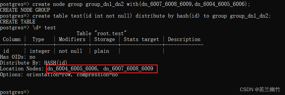
create table test1(id int not null)
DISTRIBUTE BY RANGE(id)(
slice s1 values less than(10) datanode dn_6004_6005_6006,
slice s2 values less than(20) datanode dn_6007_6008_6009,
slice s3 values less than(30) datanode dn_6001_6002_6003,
slice s4 values less than(40) datanode dn_6001_6002_6003
);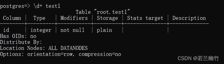
- 给
test表准备数据insert into test values(1),(2),(3),(4); test表的数据分布查询execute direct on(dn_6001_6002_6003) 'select * from test'; execute direct on(dn_6004_6005_6006) 'select * from test'; execute direct on(dn_6007_6008_6009) 'select * from test';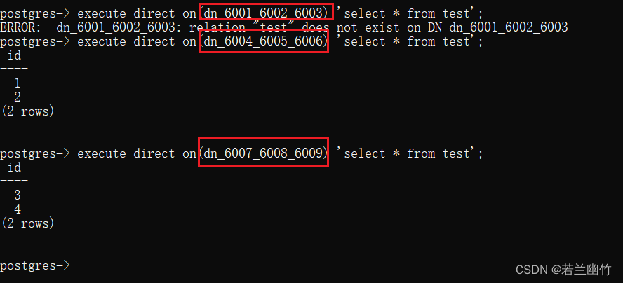
注意:这里的test表在创建时指定了所属node group,所以该表只在在两个节点上存在。
-
test表的数据分布情况select b.node_name,a.count from(select xc_node_id,count(*) from test group by xc_node_id) a,pgxc_node b where a.xc_node_id=b.node_id;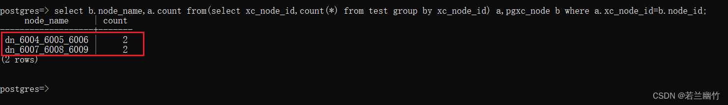
-
对
test1表进行测试insert into test1 values(1),(10),(20),(30),(35),(39); execute direct on(dn_6001_6002_6003) 'select * from test1'; execute direct on(dn_6004_6005_6006) 'select * from test1'; execute direct on(dn_6007_6008_6009) 'select * from test1';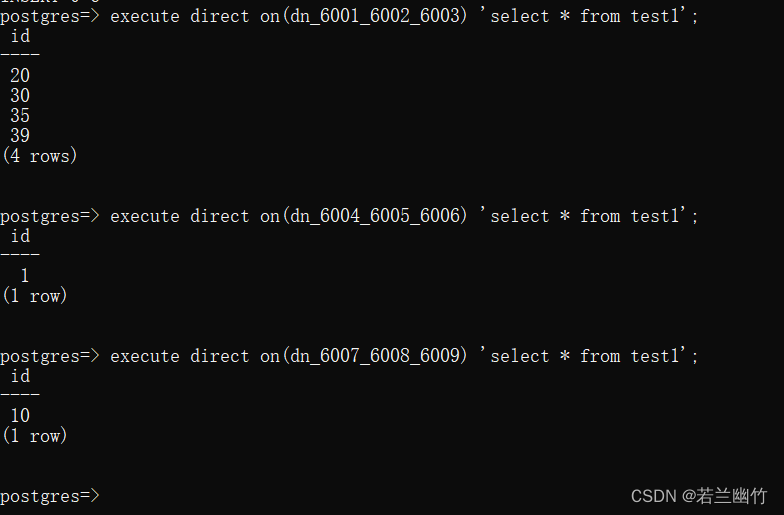
test1是按照range分片,得出重要结论:分片的范围是左闭右开的区间即"[ )"。
test1表的数据分布情况:select b.node_name,a.count from(select xc_node_id,count(*) from test1 group by xc_node_id) a,pgxc_node b where a.xc_node_id=b.node_id;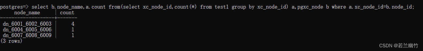
- 查询节点名称
-
数据分区示例
-
创建分片分区表
create table test_part(id int not null,age int)
DISTRIBUTE BY RANGE(id)(
slice s1 values less than(10) datanode dn_6001_6002_6003,
slice s2 values less than(20) datanode dn_6004_6005_6006,
slice s3 values less than(30) datanode dn_6007_6008_6009,
slice s4 values less than(40) datanode dn_6007_6008_6009
)
PARTITION BY RANGE(age)(
PARTITION p1 values less than(10),
PARTITION p2 values less than(20),
PARTITION p3 values less than(30),
PARTITION p4 values less than(40)
);
查看表结构:

插入测试数据:insert into test_part values(1,5),(2,9),(10,10),(19,19),(20,20),(30,30);数据分布查询:
execute direct on(dn_6001_6002_6003) 'select * from test_part';
execute direct on(dn_6004_6005_6006) 'select * from test_part';
execute direct on(dn_6007_6008_6009) 'select * from test_part';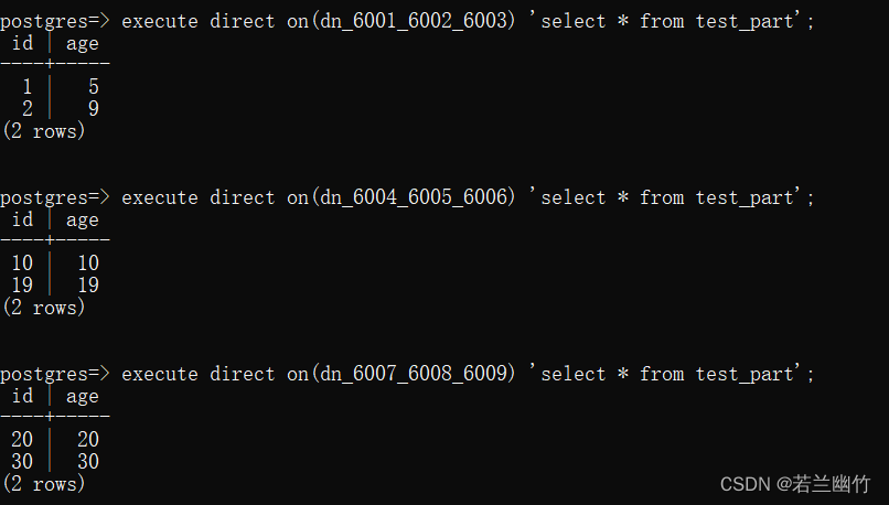
test_part表的数据分布情况:select b.node_name,a.count from(select xc_node_id,count(*) from test_part group by xc_node_id) a,pgxc_node b where a.xc_node_id=b.node_id;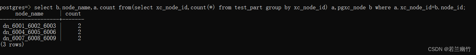
-
由此,我们可以看出GaussDB中表是按照分片进行存储,且可在分片下进行分区存储。


 3272
3272


 被折叠的 条评论
为什么被折叠?
被折叠的 条评论
为什么被折叠?
 到【灌水乐园】发言


