


In [1]:
# 导入一些需要用到的包
import pandas as pd
import numpy as np
import matplotlib as mpl
import matplotlib.pyplot as plt
%matplotlib inline

# 配置 pandas
pd.set_option('display.notebook_repr_html', False)
pd.set_option('display.max_columns', 20)
pd.set_option('display.max_rows', 25)
In [2]:
plt.plot(np.random.normal(size=100), np.random.normal(size=100), 'ro')
Out[2]:
[<matplotlib.lines.Line2D at 0x7f27e30e08d0>]
![]()
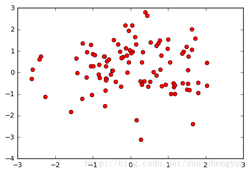
上图绘制了两组来自正态分布的随机数的散点图,“ro”是一个缩写参数,表示用“红色圆圈”绘图。这种绘图很简单,我们可以进一步通过拆分绘图流程来得到更加复杂的图像。
In [3]:
with mpl.rc_context(rc={'font.family': 'serif', 'font.weight': 'bold', 'font.size': 8}):
    fig = plt.figure(figsize=(6,3))
    ax1 = fig.add_subplot(121)
    ax1.set_xlabel('some random numbers')
    ax1.set_ylabel('more random numbers')
    ax1.set_title("Random scatterplot")
    plt.plot(np.random.normal(size=100), np.random.normal(size=100), 'r.')
    ax2 = fig.add_subplot(122)
    plt.hist(np.random.normal(size=100), bins=15)
    ax2.set_xlabel('sample')
    ax2.set_ylabel('cumulative sum')
    ax2.set_title("Normal distrubution")
    plt.tight_layout()
    plt.savefig("normalvars.png", dpi=150)
![]()
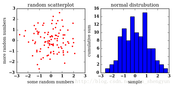
fig = plt.figure(figsize=(6,3)),定义一个长为6宽为3英寸的画布
ax1 = fig.add_subplot(121),将画布分为1行2列,从左到右从上到下取第1块
matplotlib 是一个相对初级的绘图包,直接输出的结果布局并不是十分美观,但是使用者可以通过很多种灵活的方式来调试输出的图像。
相对于 matplotlib 来讲,Pandas 支持 DataFrame 和 Series 两种比较高级的数据结构,可以想象得到用其绘制出图像的形式。
In [4]:
normals = pd.Series(np.random.normal(size=10))
normals.plot()
Out[4]:
<matplotlib.axes._subplots.AxesSubplot at 0x7f27e30f23d0>
![]()
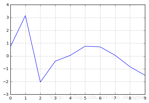
可以发现,默认绘制的是折线图,并且有灰色的网格线。当然,这些都可以修改。
In [5]:
normals.cumsum().plot(grid=False)
Out[5]:
<matplotlib.axes._subplots.AxesSubplot at 0x7f27df5a6090>

![]()
对于 DataFrame 结构的数据,也可以进行类似的操作:
In [6]:
variables = pd.DataFrame({'normal': np.random.normal(size=100),
                       'gamma': np.random.gamma(1, size=100),
                       'poisson': np.random.poisson(size=100)})
variables.cumsum(0).plot()
Out[6]:
<matplotlib.axes._subplots.AxesSubplot at 0x7f27df4aa410>

![]()
Pandas 还支持这样的操作:利用参数“subplots”绘制 DataFrame 中每个序列对应的子图
In [7]:
variables.cumsum(0).plot(subplots=True)
Out[7]:
array([<matplotlib.axes._subplots.AxesSubplot object at 0x7f27df48c750>,
       <matplotlib.axes._subplots.AxesSubplot object at 0x7f27df321990>,
       <matplotlib.axes._subplots.AxesSubplot object at 0x7f27df2a66d0>], dtype=object)

![]()
或者,我们也可以绘制双坐标轴,将某些序列用次坐标轴展示,这样可以展示更多细节并且图像中没有过多空白。
In [8]:
variables.cumsum(0).plot(secondary_y='normal')
Out[8]:
<matplotlib.axes._subplots.AxesSubplot at 0x7f27df4b4910>

![]()
如果你有更多的绘图要求,也可以直接利用 matplotlib 的 “subplots” 方法,手动设置图像位置:
In [9]:
fig, axes = plt.subplots(nrows=1, ncols=3, figsize=(12, 4))
for i,var in enumerate(['normal','gamma','poisson']):
    variables[var].cumsum(0).plot(ax=axes[i], title=var)
axes[0].set_ylabel('cumulative sum')
Out[9]:
<matplotlib.text.Text at 0x7f27deffc3d0>

![]() In [10]:
In [10]:
titanic = pd.read_excel("data/titanic.xls", "titanic")
titanic.head()
Out[10]:
   pclass  survived                                             name     sex  \
0       1         1                    Allen, Miss. Elisabeth Walton  female
1       1         1                   Allison, Master. Hudson Trevor    male
2       1         0                     Allison, Miss. Helen Loraine  female
3       1         0             Allison, Mr. Hudson Joshua Creighton    male
4       1         0  Allison, Mrs. Hudson J C (Bessie Waldo Daniels)  female

       age  sibsp  parch  ticket      fare    cabin embarked boat   body  \
0  29.0000      0      0   24160  211.3375       B5        S    2    NaN
1   0.9167      1      2  113781  151.5500  C22 C26        S   11    NaN
2   2.0000      1      2  113781  151.5500  C22 C26        S  NaN    NaN
3  30.0000      1      2  113781  151.5500  C22 C26        S  NaN  135.0
4  25.0000      1      2  113781  151.5500  C22 C26        S  NaN    NaN

                         home.dest
0                     St Louis, MO
1  Montreal, PQ / Chesterville, ON
2  Montreal, PQ / Chesterville, ON
3  Montreal, PQ / Chesterville, ON
4  Montreal, PQ / Chesterville, ON
In [11]:
titanic.groupby('pclass').survived.sum().plot(kind='bar')
Out[11]:
<matplotlib.axes._subplots.AxesSubplot at 0x7f27deaecc50>

![]() In [12]:
In [12]:
titanic.groupby(['sex','pclass']).survived.sum().plot(kind='barh')
Out[12]:
<matplotlib.axes._subplots.AxesSubplot at 0x7f27deb28250>

![]() In [13]:
In [13]:
death_counts = pd.crosstab([titanic.pclass, titanic.sex], titanic.survived.astype(bool))
death_counts.plot(kind='bar', stacked=True, color=['black','gold'], grid=False)
Out[13]:
<matplotlib.axes._subplots.AxesSubplot at 0x7f27dea6d290>

![]()
还可以通过除以该组的总人数来对比不同组之间的存活率
In [14]:
death_counts.div(death_counts.sum(1).astype(float), axis=0).plot(kind='barh', stacked=True, color=['black','gold'])
Out[14]:
<matplotlib.axes._subplots.AxesSubplot at 0x7f27de9847d0>

![]() In [15]:
In [15]:
titanic.fare.hist(grid=False)
Out[15]:
<matplotlib.axes._subplots.AxesSubplot at 0x7f27de7a5190>

![]()
“hist”方法默认将连续票价划分为 10 个区间,我们可以通过设置参数“bins”来设定区间个数(或者说设定直方图的宽度):
In [16]:
titanic.fare.hist(bins=30)
Out[16]:
<matplotlib.axes._subplots.AxesSubplot at 0x7f27de7eca50>

![]()
有很多种计算最优区间个数的算法,且都会一定程度的随观测值个数变化。
In [17]:
sturges = lambda n: int(np.log2(n) + 1)
square_root = lambda n: int(np.sqrt(n))
from scipy.stats import kurtosis
doanes = lambda data: int(1 + np.log(len(data)) + np.log(1 + kurtosis(data) * (len(data) / 6.) ** 0.5))

n = len(titanic)
sturges(n), square_root(n), doanes(titanic.fare.dropna())
Out[17]:
(11, 36, 14)
In [18]:
titanic.fare.hist(bins=doanes(titanic.fare.dropna()))
Out[18]:
<matplotlib.axes._subplots.AxesSubplot at 0x7f27de69bc10>
![]()
和直方图类似,密度图也描述了数据的分布情况,可以看成将直方图区间无限细分后形成的平滑曲线。设置“plot”方法的参数 kind='kde',即可绘制密度图,其中 'kde' 表示“kernel density estimate”。
In [19]:
titanic.fare.dropna().plot(kind='kde', xlim=(0,600))
Out[19]:
<matplotlib.axes._subplots.AxesSubplot at 0x7f27d810a950>

![]() 通常,直方图和密度图会绘制在同一张图里:
In [20]:
通常,直方图和密度图会绘制在同一张图里:
In [20]:
titanic.fare.hist(bins=doanes(titanic.fare.dropna()), normed=True, color='lightseagreen')
titanic.fare.dropna().plot(kind='kde', xlim=(0,600), style='r--')
Out[20]:
<matplotlib.axes._subplots.AxesSubplot at 0x7f27d8103350>

![]()
这里我们需要通过设置参数“normed=True”将直方图标准化处理,因为概率密度分布是标准化的,
In [21]:
titanic.boxplot(column='fare', by='pclass', grid=False)
Out[21]:
<matplotlib.axes._subplots.AxesSubplot at 0x7f27d7fc8590>
![]()
可以将箱线图看成数据的分布图,图中“+”的点表示异常值。
可以将实际数据同时展示在箱线图中来丰富图像信息,这种做法比较适合观测值较少的数据集。
In [22]:
bp = titanic.boxplot(column='age', by='pclass', grid=False)
for i in [1,2,3]:
    y = titanic.age[titanic.pclass==i].dropna()
    # 通过设置随机值,使观测值在x轴方向不重叠
    x = np.random.normal(i, 0.04, size=len(y))
    plt.plot(x, y, 'r.', alpha=0.2)
![]()
当数据分布非常稠密时,有以下两种方式来增强图形的可读性: 1、降低透明度,使数据点半透明 2、增加数据点 x 轴方向的随机距离,减少数据点之间的重叠
一个和箱线图相近但远不及箱线图的图像叫做“dynamite”图,本质上就是给出标准偏差的柱状图
In [23]:
titanic.groupby('pclass')['fare'].mean().plot(kind='bar', yerr=titanic.groupby('pclass')['fare'].std())
Out[23]:
<matplotlib.axes._subplots.AxesSubplot at 0x7f27d7d22490>
![]()
为什么我们比较少用这种绘图方式呢?
- 柱状图覆盖的区域并没有实际含义
- 信息含量低,只反映了6个数值:三个均值和三个标准差
- 掩藏了原始数据的真实信息
相比之下,箱线图是更好的选择。
In [24]:
data1 = [150, 155, 175, 200, 245, 255, 395, 300, 305, 320, 375, 400, 420, 430, 440]
data2 = [225, 380]

fake_data = pd.DataFrame([data1, data2]).transpose()
p = fake_data.mean().plot(kind='bar', yerr=fake_data.std(), grid=False)
![]() In [25]:
In [25]:
fake_data = pd.DataFrame([data1, data2]).transpose()
p = fake_data.mean().plot(kind='bar', yerr=fake_data.std(), grid=False)
x1, x2 = p.xaxis.get_majorticklocs()
plt.plot(np.random.normal(x1, 0.01, size=len(data1)), data1, 'ro')
plt.plot([x2]*len(data2), data2, 'ro')
Out[25]:
[<matplotlib.lines.Line2D at 0x7f27d7c2c910>]
![]() In [26]:
In [26]:
baseball = pd.read_csv("data/baseball.csv")
baseball.head()
Out[26]:
      id     player  year  stint team  lg   g  ab  r   h  ...   rbi   sb   cs  \
0  88641  womacto01  2006      2  CHN  NL  19  50  6  14  ...   2.0  1.0  1.0
1  88643  schilcu01  2006      1  BOS  AL  31   2  0   1  ...   0.0  0.0  0.0
2  88645  myersmi01  2006      1  NYA  AL  62   0  0   0  ...   0.0  0.0  0.0
3  88649  helliri01  2006      1  MIL  NL  20   3  0   0  ...   0.0  0.0  0.0
4  88650  johnsra05  2006      1  NYA  AL  33   6  0   1  ...   0.0  0.0  0.0

   bb   so  ibb  hbp   sh   sf  gidp
0   4  4.0  0.0  0.0  3.0  0.0   0.0
1   0  1.0  0.0  0.0  0.0  0.0   0.0
2   0  0.0  0.0  0.0  0.0  0.0   0.0
3   0  2.0  0.0  0.0  0.0  0.0   0.0
4   0  4.0  0.0  0.0  0.0  0.0   0.0

[5 rows x 23 columns]
在探索变量之间的关系=时,可以绘制散点图。Series 或者 DataFrame 结构的数据并没有相应的绘制散点图的方法,必须使用 matplotlib 的“scatter”函数。
In [27]:
plt.scatter(baseball.ab, baseball.h)
plt.xlim(0, 700); plt.ylim(0, 200)
Out[27]:
(0, 200)
![]()
可以通过赋予样本点不同的大小和颜色来展示更多的信息。
In [28]:
plt.scatter(baseball.ab, baseball.h, s=baseball.hr*10, alpha=0.5)
plt.xlim(0, 700); plt.ylim(0, 200)
Out[28]:
(0, 200)
![]() In [29]:
In [29]:
plt.scatter(baseball.ab, baseball.h, c=baseball.hr, s=40, cmap='hot')
plt.xlim(0, 700); plt.ylim(0, 200);
![]()
可以使用“scatter_matrix”函数同时展示多个变量之间的散点图,最终会生成一个两两对应的散点图矩阵,可以选择在对角线展示直方图或者密度图。
In [30]:
_ = pd.scatter_matrix(baseball.loc[:,'r':'sb'], figsize=(12,8), diagonal='kde')
![]()
下面利用泰坦尼克数据集绘制一个栅栏图来同时展示 4 个变量之间的关系,有以下 4 个步骤: 1、创建一个仅和数据集中两个变量有关的“RPlot” 2、利用“passenger class ”和“sex”两个变量的不同取值最为条件区分,添加网格 3、增加用于可视化的实际数据 4、可视化展示
In [31]:
from pandas.tools.rplot import *

titanic = titanic[titanic.age.notnull() & titanic.fare.notnull()]

tp = RPlot(titanic, x='age')
tp.add(TrellisGrid(['pclass', 'sex']))
tp.add(GeomDensity())
_ = tp.render(plt.gcf())
/home/datartisan/.pyenv/versions/2.7.12/envs/datacademy-lesson-27/lib/python2.7/site-packages/ipykernel/__main__.py:1: FutureWarning:
The rplot trellis plotting interface is deprecated and will be removed in a future version. We refer to external packages like seaborn for similar but more refined functionality.

See our docs http://pandas.pydata.org/pandas-docs/stable/visualization.html#rplot for some example how to convert your existing code to these packages.
  if __name__ == '__main__':
![]()
利用张力障碍数据集,将“age”和“twstrs”两个变量之间的关系作为“week”和“treat”两个变量的函数,通过绘制散点图,我们可以同时探索不同情境下二者之间的关系,并进行拟合:
In [32]:
cdystonia = pd.read_csv("data/cdystonia.csv", index_col=None)
cdystonia.head()
Out[32]:
   patient  obs  week  site  id  treat  age sex  twstrs
0        1    1     0     1   1  5000U   65   F      32
1        1    2     2     1   1  5000U   65   F      30
2        1    3     4     1   1  5000U   65   F      24
3        1    4     8     1   1  5000U   65   F      37
4        1    5    12     1   1  5000U   65   F      39
In [33]:
plt.figure(figsize=(12,12))
bbp = RPlot(cdystonia, x='age', y='twstrs')
bbp.add(TrellisGrid(['week', 'treat']))
bbp.add(GeomScatter())
bbp.add(GeomPolyFit(degree=2))
_ = bbp.render(plt.gcf())
![]()
RPlot 不仅仅可以被用来绘制栅栏图,也可以通过使用不同的颜色、大小、形状等将多个变量绘制在一起。
In [34]:
cdystonia['site'] = cdystonia.site.astype(float)
In [35]:
plt.figure(figsize=(6,6))
cp = RPlot(cdystonia, x='age', y='twstrs')
cp.add(GeomPoint(colour=ScaleGradient('site', colour1=(1.0, 1.0, 0.5), colour2=(1.0, 0.0, 0.0)),
            size=ScaleSize('week', min_size=10.0, max_size=200.0),
            shape=ScaleShape('treat')))
_ = cp.render(plt.gcf())
/home/datartisan/.pyenv/versions/2.7.12/envs/datacademy-lesson-27/lib/python2.7/site-packages/pandas/tools/rplot.py:167: FutureWarning: iget(i) is deprecated. Please use .iloc[i] or .iat[i]
  x = data[self.column].iget(index)
/home/datartisan/.pyenv/versions/2.7.12/envs/datacademy-lesson-27/lib/python2.7/site-packages/pandas/tools/rplot.py:66: FutureWarning: iget(i) is deprecated. Please use .iloc[i] or .iat[i]
  x = data[self.column].iget(index)
/home/datartisan/.pyenv/versions/2.7.12/envs/datacademy-lesson-27/lib/python2.7/site-packages/pandas/tools/rplot.py:208: FutureWarning: iget(i) is deprecated. Please use .iloc[i] or .iat[i]
  x = data[self.column].iget(index)
![]()
![]()
In [1]:
# 导入一些需要用到的包
import pandas as pd
import numpy as np
import matplotlib as mpl
import matplotlib.pyplot as plt
%matplotlib inline
# 配置 pandas
pd.set_option('display.notebook_repr_html', False)
pd.set_option('display.max_columns', 20)
pd.set_option('display.max_rows', 25)
In [2]:
plt.plot(np.random.normal(size=100), np.random.normal(size=100), 'ro')
Out[2]:
[<matplotlib.lines.Line2D at 0x7f27e30e08d0>]
![]()
上图绘制了两组来自正态分布的随机数的散点图,“ro”是一个缩写参数,表示用“红色圆圈”绘图。这种绘图很简单,我们可以进一步通过拆分绘图流程来得到更加复杂的图像。
In [3]:
with mpl.rc_context(rc={'font.family': 'serif', 'font.weight': 'bold', 'font.size': 8}):
fig = plt.figure(figsize=(6,3))
ax1 = fig.add_subplot(121)
ax1.set_xlabel('some random numbers')
ax1.set_ylabel('more random numbers')
ax1.set_title("Random scatterplot")
plt.plot(np.random.normal(size=100), np.random.normal(size=100), 'r.')
ax2 = fig.add_subplot(122)
plt.hist(np.random.normal(size=100), bins=15)
ax2.set_xlabel('sample')
ax2.set_ylabel('cumulative sum')
ax2.set_title("Normal distrubution")
plt.tight_layout()
plt.savefig("normalvars.png", dpi=150)
![]()
fig = plt.figure(figsize=(6,3)),定义一个长为6宽为3英寸的画布
ax1 = fig.add_subplot(121),将画布分为1行2列,从左到右从上到下取第1块
matplotlib 是一个相对初级的绘图包,直接输出的结果布局并不是十分美观,但是使用者可以通过很多种灵活的方式来调试输出的图像。
相对于 matplotlib 来讲,Pandas 支持 DataFrame 和 Series 两种比较高级的数据结构,可以想象得到用其绘制出图像的形式。
In [4]:
normals = pd.Series(np.random.normal(size=10))
normals.plot()
Out[4]:
<matplotlib.axes._subplots.AxesSubplot at 0x7f27e30f23d0>
![]()
可以发现,默认绘制的是折线图,并且有灰色的网格线。当然,这些都可以修改。
In [5]:
normals.cumsum().plot(grid=False)
Out[5]:
<matplotlib.axes._subplots.AxesSubplot at 0x7f27df5a6090>
![]()
对于 DataFrame 结构的数据,也可以进行类似的操作:
In [6]:
variables = pd.DataFrame({'normal': np.random.normal(size=100),
'gamma': np.random.gamma(1, size=100),
'poisson': np.random.poisson(size=100)})
variables.cumsum(0).plot()
Out[6]:
<matplotlib.axes._subplots.AxesSubplot at 0x7f27df4aa410>
![]()
Pandas 还支持这样的操作:利用参数“subplots”绘制 DataFrame 中每个序列对应的子图
In [7]:
variables.cumsum(0).plot(subplots=True)
Out[7]:
array([<matplotlib.axes._subplots.AxesSubplot object at 0x7f27df48c750>,
<matplotlib.axes._subplots.AxesSubplot object at 0x7f27df321990>,
<matplotlib.axes._subplots.AxesSubplot object at 0x7f27df2a66d0>], dtype=object)
![]()
或者,我们也可以绘制双坐标轴,将某些序列用次坐标轴展示,这样可以展示更多细节并且图像中没有过多空白。
In [8]:
variables.cumsum(0).plot(secondary_y='normal')
Out[8]:
<matplotlib.axes._subplots.AxesSubplot at 0x7f27df4b4910>
![]()
如果你有更多的绘图要求,也可以直接利用 matplotlib 的 “subplots” 方法,手动设置图像位置:
In [9]:
fig, axes = plt.subplots(nrows=1, ncols=3, figsize=(12, 4))
for i,var in enumerate(['normal','gamma','poisson']):
variables[var].cumsum(0).plot(ax=axes[i], title=var)
axes[0].set_ylabel('cumulative sum')
Out[9]:
<matplotlib.text.Text at 0x7f27deffc3d0>
![]() In [10]:
In [10]:
titanic = pd.read_excel("data/titanic.xls", "titanic")
titanic.head()
Out[10]:
pclass survived name sex \
0 1 1 Allen, Miss. Elisabeth Walton female
1 1 1 Allison, Master. Hudson Trevor male
2 1 0 Allison, Miss. Helen Loraine female
3 1 0 Allison, Mr. Hudson Joshua Creighton male
4 1 0 Allison, Mrs. Hudson J C (Bessie Waldo Daniels) female
age sibsp parch ticket fare cabin embarked boat body \
0 29.0000 0 0 24160 211.3375 B5 S 2 NaN
1 0.9167 1 2 113781 151.5500 C22 C26 S 11 NaN
2 2.0000 1 2 113781 151.5500 C22 C26 S NaN NaN
3 30.0000 1 2 113781 151.5500 C22 C26 S NaN 135.0
4 25.0000 1 2 113781 151.5500 C22 C26 S NaN NaN
home.dest
0 St Louis, MO
1 Montreal, PQ / Chesterville, ON
2 Montreal, PQ / Chesterville, ON
3 Montreal, PQ / Chesterville, ON
4 Montreal, PQ / Chesterville, ON
In [11]:
titanic.groupby('pclass').survived.sum().plot(kind='bar')
Out[11]:
<matplotlib.axes._subplots.AxesSubplot at 0x7f27deaecc50>
![]() In [12]:
In [12]:
titanic.groupby(['sex','pclass']).survived.sum().plot(kind='barh')
Out[12]:
<matplotlib.axes._subplots.AxesSubplot at 0x7f27deb28250>
![]() In [13]:
In [13]:
death_counts = pd.crosstab([titanic.pclass, titanic.sex], titanic.survived.astype(bool))
death_counts.plot(kind='bar', stacked=True, color=['black','gold'], grid=False)
Out[13]:
<matplotlib.axes._subplots.AxesSubplot at 0x7f27dea6d290>
![]()
还可以通过除以该组的总人数来对比不同组之间的存活率
In [14]:
death_counts.div(death_counts.sum(1).astype(float), axis=0).plot(kind='barh', stacked=True, color=['black','gold'])
Out[14]:
<matplotlib.axes._subplots.AxesSubplot at 0x7f27de9847d0>
![]() In [15]:
In [15]:
titanic.fare.hist(grid=False)
Out[15]:
<matplotlib.axes._subplots.AxesSubplot at 0x7f27de7a5190>
![]()
“hist”方法默认将连续票价划分为 10 个区间,我们可以通过设置参数“bins”来设定区间个数(或者说设定直方图的宽度):
In [16]:
titanic.fare.hist(bins=30)
Out[16]:
<matplotlib.axes._subplots.AxesSubplot at 0x7f27de7eca50>
![]()
有很多种计算最优区间个数的算法,且都会一定程度的随观测值个数变化。
In [17]:
sturges = lambda n: int(np.log2(n) + 1)
square_root = lambda n: int(np.sqrt(n))
from scipy.stats import kurtosis
doanes = lambda data: int(1 + np.log(len(data)) + np.log(1 + kurtosis(data) * (len(data) / 6.) ** 0.5))
n = len(titanic)
sturges(n), square_root(n), doanes(titanic.fare.dropna())
Out[17]:
(11, 36, 14)
In [18]:
titanic.fare.hist(bins=doanes(titanic.fare.dropna()))
Out[18]:
<matplotlib.axes._subplots.AxesSubplot at 0x7f27de69bc10>
![]()
和直方图类似,密度图也描述了数据的分布情况,可以看成将直方图区间无限细分后形成的平滑曲线。设置“plot”方法的参数 kind='kde',即可绘制密度图,其中 'kde' 表示“kernel density estimate”。
In [19]:
titanic.fare.dropna().plot(kind='kde', xlim=(0,600))
Out[19]:
<matplotlib.axes._subplots.AxesSubplot at 0x7f27d810a950>
![]() 通常,直方图和密度图会绘制在同一张图里:
In [20]:
通常,直方图和密度图会绘制在同一张图里:
In [20]:
titanic.fare.hist(bins=doanes(titanic.fare.dropna()), normed=True, color='lightseagreen')
titanic.fare.dropna().plot(kind='kde', xlim=(0,600), style='r--')
Out[20]:
<matplotlib.axes._subplots.AxesSubplot at 0x7f27d8103350>
![]()
这里我们需要通过设置参数“normed=True”将直方图标准化处理,因为概率密度分布是标准化的,
In [21]:
titanic.boxplot(column='fare', by='pclass', grid=False)
Out[21]:
<matplotlib.axes._subplots.AxesSubplot at 0x7f27d7fc8590>
![]()
可以将箱线图看成数据的分布图,图中“+”的点表示异常值。
可以将实际数据同时展示在箱线图中来丰富图像信息,这种做法比较适合观测值较少的数据集。
In [22]:
bp = titanic.boxplot(column='age', by='pclass', grid=False)
for i in [1,2,3]:
y = titanic.age[titanic.pclass==i].dropna()
# 通过设置随机值,使观测值在x轴方向不重叠
x = np.random.normal(i, 0.04, size=len(y))
plt.plot(x, y, 'r.', alpha=0.2)
![]()
当数据分布非常稠密时,有以下两种方式来增强图形的可读性: 1、降低透明度,使数据点半透明 2、增加数据点 x 轴方向的随机距离,减少数据点之间的重叠
一个和箱线图相近但远不及箱线图的图像叫做“dynamite”图,本质上就是给出标准偏差的柱状图
In [23]:
titanic.groupby('pclass')['fare'].mean().plot(kind='bar', yerr=titanic.groupby('pclass')['fare'].std())
Out[23]:
<matplotlib.axes._subplots.AxesSubplot at 0x7f27d7d22490>
![]()
为什么我们比较少用这种绘图方式呢?
- 柱状图覆盖的区域并没有实际含义
- 信息含量低,只反映了6个数值:三个均值和三个标准差
- 掩藏了原始数据的真实信息
相比之下,箱线图是更好的选择。
In [24]:
data1 = [150, 155, 175, 200, 245, 255, 395, 300, 305, 320, 375, 400, 420, 430, 440]
data2 = [225, 380]
fake_data = pd.DataFrame([data1, data2]).transpose()
p = fake_data.mean().plot(kind='bar', yerr=fake_data.std(), grid=False)
![]() In [25]:
In [25]:
fake_data = pd.DataFrame([data1, data2]).transpose()
p = fake_data.mean().plot(kind='bar', yerr=fake_data.std(), grid=False)
x1, x2 = p.xaxis.get_majorticklocs()
plt.plot(np.random.normal(x1, 0.01, size=len(data1)), data1, 'ro')
plt.plot([x2]*len(data2), data2, 'ro')
Out[25]:
[<matplotlib.lines.Line2D at 0x7f27d7c2c910>]
![]() In [26]:
In [26]:
baseball = pd.read_csv("data/baseball.csv")
baseball.head()
Out[26]:
id player year stint team lg g ab r h ... rbi sb cs \
0 88641 womacto01 2006 2 CHN NL 19 50 6 14 ... 2.0 1.0 1.0
1 88643 schilcu01 2006 1 BOS AL 31 2 0 1 ... 0.0 0.0 0.0
2 88645 myersmi01 2006 1 NYA AL 62 0 0 0 ... 0.0 0.0 0.0
3 88649 helliri01 2006 1 MIL NL 20 3 0 0 ... 0.0 0.0 0.0
4 88650 johnsra05 2006 1 NYA AL 33 6 0 1 ... 0.0 0.0 0.0
bb so ibb hbp sh sf gidp
0 4 4.0 0.0 0.0 3.0 0.0 0.0
1 0 1.0 0.0 0.0 0.0 0.0 0.0
2 0 0.0 0.0 0.0 0.0 0.0 0.0
3 0 2.0 0.0 0.0 0.0 0.0 0.0
4 0 4.0 0.0 0.0 0.0 0.0 0.0
[5 rows x 23 columns]
在探索变量之间的关系=时,可以绘制散点图。Series 或者 DataFrame 结构的数据并没有相应的绘制散点图的方法,必须使用 matplotlib 的“scatter”函数。
In [27]:
plt.scatter(baseball.ab, baseball.h)
plt.xlim(0, 700); plt.ylim(0, 200)
Out[27]:
(0, 200)
![]()
可以通过赋予样本点不同的大小和颜色来展示更多的信息。
In [28]:
plt.scatter(baseball.ab, baseball.h, s=baseball.hr*10, alpha=0.5)
plt.xlim(0, 700); plt.ylim(0, 200)
Out[28]:
(0, 200)
![]() In [29]:
In [29]:
plt.scatter(baseball.ab, baseball.h, c=baseball.hr, s=40, cmap='hot')
plt.xlim(0, 700); plt.ylim(0, 200);
![]()
可以使用“scatter_matrix”函数同时展示多个变量之间的散点图,最终会生成一个两两对应的散点图矩阵,可以选择在对角线展示直方图或者密度图。
In [30]:
_ = pd.scatter_matrix(baseball.loc[:,'r':'sb'], figsize=(12,8), diagonal='kde')
![]()
下面利用泰坦尼克数据集绘制一个栅栏图来同时展示 4 个变量之间的关系,有以下 4 个步骤: 1、创建一个仅和数据集中两个变量有关的“RPlot” 2、利用“passenger class ”和“sex”两个变量的不同取值最为条件区分,添加网格 3、增加用于可视化的实际数据 4、可视化展示
In [31]:
from pandas.tools.rplot import *
titanic = titanic[titanic.age.notnull() & titanic.fare.notnull()]
tp = RPlot(titanic, x='age')
tp.add(TrellisGrid(['pclass', 'sex']))
tp.add(GeomDensity())
_ = tp.render(plt.gcf())
/home/datartisan/.pyenv/versions/2.7.12/envs/datacademy-lesson-27/lib/python2.7/site-packages/ipykernel/__main__.py:1: FutureWarning:
The rplot trellis plotting interface is deprecated and will be removed in a future version. We refer to external packages like seaborn for similar but more refined functionality.
See our docs http://pandas.pydata.org/pandas-docs/stable/visualization.html#rplot for some example how to convert your existing code to these packages.
if __name__ == '__main__':
![]()
利用张力障碍数据集,将“age”和“twstrs”两个变量之间的关系作为“week”和“treat”两个变量的函数,通过绘制散点图,我们可以同时探索不同情境下二者之间的关系,并进行拟合:
In [32]:
cdystonia = pd.read_csv("data/cdystonia.csv", index_col=None)
cdystonia.head()
Out[32]:
patient obs week site id treat age sex twstrs
0 1 1 0 1 1 5000U 65 F 32
1 1 2 2 1 1 5000U 65 F 30
2 1 3 4 1 1 5000U 65 F 24
3 1 4 8 1 1 5000U 65 F 37
4 1 5 12 1 1 5000U 65 F 39
In [33]:
plt.figure(figsize=(12,12))
bbp = RPlot(cdystonia, x='age', y='twstrs')
bbp.add(TrellisGrid(['week', 'treat']))
bbp.add(GeomScatter())
bbp.add(GeomPolyFit(degree=2))
_ = bbp.render(plt.gcf())
![]()
RPlot 不仅仅可以被用来绘制栅栏图,也可以通过使用不同的颜色、大小、形状等将多个变量绘制在一起。
In [34]:
cdystonia['site'] = cdystonia.site.astype(float)
In [35]:
plt.figure(figsize=(6,6))
cp = RPlot(cdystonia, x='age', y='twstrs')
cp.add(GeomPoint(colour=ScaleGradient('site', colour1=(1.0, 1.0, 0.5), colour2=(1.0, 0.0, 0.0)),
size=ScaleSize('week', min_size=10.0, max_size=200.0),
shape=ScaleShape('treat')))
_ = cp.render(plt.gcf())
/home/datartisan/.pyenv/versions/2.7.12/envs/datacademy-lesson-27/lib/python2.7/site-packages/pandas/tools/rplot.py:167: FutureWarning: iget(i) is deprecated. Please use .iloc[i] or .iat[i]
x = data[self.column].iget(index)
/home/datartisan/.pyenv/versions/2.7.12/envs/datacademy-lesson-27/lib/python2.7/site-packages/pandas/tools/rplot.py:66: FutureWarning: iget(i) is deprecated. Please use .iloc[i] or .iat[i]
x = data[self.column].iget(index)
/home/datartisan/.pyenv/versions/2.7.12/envs/datacademy-lesson-27/lib/python2.7/site-packages/pandas/tools/rplot.py:208: FutureWarning: iget(i) is deprecated. Please use .iloc[i] or .iat[i]
x = data[self.column].iget(index)
![]()
# 导入一些需要用到的包
import pandas as pd
import numpy as np
import matplotlib as mpl
import matplotlib.pyplot as plt
%matplotlib inline
# 配置 pandas
pd.set_option('display.notebook_repr_html', False)
pd.set_option('display.max_columns', 20)
pd.set_option('display.max_rows', 25)
plt.plot(np.random.normal(size=100), np.random.normal(size=100), 'ro')
[<matplotlib.lines.Line2D at 0x7f27e30e08d0>]
上图绘制了两组来自正态分布的随机数的散点图,“ro”是一个缩写参数,表示用“红色圆圈”绘图。这种绘图很简单,我们可以进一步通过拆分绘图流程来得到更加复杂的图像。
with mpl.rc_context(rc={'font.family': 'serif', 'font.weight': 'bold', 'font.size': 8}):
fig = plt.figure(figsize=(6,3))
ax1 = fig.add_subplot(121)
ax1.set_xlabel('some random numbers')
ax1.set_ylabel('more random numbers')
ax1.set_title("Random scatterplot")
plt.plot(np.random.normal(size=100), np.random.normal(size=100), 'r.')
ax2 = fig.add_subplot(122)
plt.hist(np.random.normal(size=100), bins=15)
ax2.set_xlabel('sample')
ax2.set_ylabel('cumulative sum')
ax2.set_title("Normal distrubution")
plt.tight_layout()
plt.savefig("normalvars.png", dpi=150)
fig = plt.figure(figsize=(6,3)),定义一个长为6宽为3英寸的画布 ax1 = fig.add_subplot(121),将画布分为1行2列,从左到右从上到下取第1块matplotlib 是一个相对初级的绘图包,直接输出的结果布局并不是十分美观,但是使用者可以通过很多种灵活的方式来调试输出的图像。
相对于 matplotlib 来讲,Pandas 支持 DataFrame 和 Series 两种比较高级的数据结构,可以想象得到用其绘制出图像的形式。
normals = pd.Series(np.random.normal(size=10))
normals.plot()
<matplotlib.axes._subplots.AxesSubplot at 0x7f27e30f23d0>
可以发现,默认绘制的是折线图,并且有灰色的网格线。当然,这些都可以修改。
normals.cumsum().plot(grid=False)
<matplotlib.axes._subplots.AxesSubplot at 0x7f27df5a6090>
对于 DataFrame 结构的数据,也可以进行类似的操作:
variables = pd.DataFrame({'normal': np.random.normal(size=100),
'gamma': np.random.gamma(1, size=100),
'poisson': np.random.poisson(size=100)})
variables.cumsum(0).plot()
<matplotlib.axes._subplots.AxesSubplot at 0x7f27df4aa410>
Pandas 还支持这样的操作:利用参数“subplots”绘制 DataFrame 中每个序列对应的子图
variables.cumsum(0).plot(subplots=True)
array([<matplotlib.axes._subplots.AxesSubplot object at 0x7f27df48c750>,
<matplotlib.axes._subplots.AxesSubplot object at 0x7f27df321990>,
<matplotlib.axes._subplots.AxesSubplot object at 0x7f27df2a66d0>], dtype=object)
或者,我们也可以绘制双坐标轴,将某些序列用次坐标轴展示,这样可以展示更多细节并且图像中没有过多空白。
variables.cumsum(0).plot(secondary_y='normal')
<matplotlib.axes._subplots.AxesSubplot at 0x7f27df4b4910>
如果你有更多的绘图要求,也可以直接利用 matplotlib 的 “subplots” 方法,手动设置图像位置:
fig, axes = plt.subplots(nrows=1, ncols=3, figsize=(12, 4))
for i,var in enumerate(['normal','gamma','poisson']):
variables[var].cumsum(0).plot(ax=axes[i], title=var)
axes[0].set_ylabel('cumulative sum')
<matplotlib.text.Text at 0x7f27deffc3d0>
titanic = pd.read_excel("data/titanic.xls", "titanic")
titanic.head()
pclass survived name sex \
0 1 1 Allen, Miss. Elisabeth Walton female
1 1 1 Allison, Master. Hudson Trevor male
2 1 0 Allison, Miss. Helen Loraine female
3 1 0 Allison, Mr. Hudson Joshua Creighton male
4 1 0 Allison, Mrs. Hudson J C (Bessie Waldo Daniels) female
age sibsp parch ticket fare cabin embarked boat body \
0 29.0000 0 0 24160 211.3375 B5 S 2 NaN
1 0.9167 1 2 113781 151.5500 C22 C26 S 11 NaN
2 2.0000 1 2 113781 151.5500 C22 C26 S NaN NaN
3 30.0000 1 2 113781 151.5500 C22 C26 S NaN 135.0
4 25.0000 1 2 113781 151.5500 C22 C26 S NaN NaN
home.dest
0 St Louis, MO
1 Montreal, PQ / Chesterville, ON
2 Montreal, PQ / Chesterville, ON
3 Montreal, PQ / Chesterville, ON
4 Montreal, PQ / Chesterville, ON
titanic.groupby('pclass').survived.sum().plot(kind='bar')
<matplotlib.axes._subplots.AxesSubplot at 0x7f27deaecc50>
titanic.groupby(['sex','pclass']).survived.sum().plot(kind='barh')
<matplotlib.axes._subplots.AxesSubplot at 0x7f27deb28250>
death_counts = pd.crosstab([titanic.pclass, titanic.sex], titanic.survived.astype(bool))
death_counts.plot(kind='bar', stacked=True, color=['black','gold'], grid=False)
<matplotlib.axes._subplots.AxesSubplot at 0x7f27dea6d290>
还可以通过除以该组的总人数来对比不同组之间的存活率
death_counts.div(death_counts.sum(1).astype(float), axis=0).plot(kind='barh', stacked=True, color=['black','gold'])
<matplotlib.axes._subplots.AxesSubplot at 0x7f27de9847d0>
titanic.fare.hist(grid=False)
<matplotlib.axes._subplots.AxesSubplot at 0x7f27de7a5190>
“hist”方法默认将连续票价划分为 10 个区间,我们可以通过设置参数“bins”来设定区间个数(或者说设定直方图的宽度):
titanic.fare.hist(bins=30)
<matplotlib.axes._subplots.AxesSubplot at 0x7f27de7eca50>
有很多种计算最优区间个数的算法,且都会一定程度的随观测值个数变化。
sturges = lambda n: int(np.log2(n) + 1)
square_root = lambda n: int(np.sqrt(n))
from scipy.stats import kurtosis
doanes = lambda data: int(1 + np.log(len(data)) + np.log(1 + kurtosis(data) * (len(data) / 6.) ** 0.5))
n = len(titanic)
sturges(n), square_root(n), doanes(titanic.fare.dropna())
(11, 36, 14)
titanic.fare.hist(bins=doanes(titanic.fare.dropna()))
<matplotlib.axes._subplots.AxesSubplot at 0x7f27de69bc10>
和直方图类似,密度图也描述了数据的分布情况,可以看成将直方图区间无限细分后形成的平滑曲线。设置“plot”方法的参数 kind='kde',即可绘制密度图,其中 'kde' 表示“kernel density estimate”。
titanic.fare.dropna().plot(kind='kde', xlim=(0,600))
<matplotlib.axes._subplots.AxesSubplot at 0x7f27d810a950>
titanic.fare.hist(bins=doanes(titanic.fare.dropna()), normed=True, color='lightseagreen')
titanic.fare.dropna().plot(kind='kde', xlim=(0,600), style='r--')
<matplotlib.axes._subplots.AxesSubplot at 0x7f27d8103350>
这里我们需要通过设置参数“normed=True”将直方图标准化处理,因为概率密度分布是标准化的,
titanic.boxplot(column='fare', by='pclass', grid=False)
<matplotlib.axes._subplots.AxesSubplot at 0x7f27d7fc8590>
可以将箱线图看成数据的分布图,图中“+”的点表示异常值。
可以将实际数据同时展示在箱线图中来丰富图像信息,这种做法比较适合观测值较少的数据集。
bp = titanic.boxplot(column='age', by='pclass', grid=False)
for i in [1,2,3]:
y = titanic.age[titanic.pclass==i].dropna()
# 通过设置随机值,使观测值在x轴方向不重叠
x = np.random.normal(i, 0.04, size=len(y))
plt.plot(x, y, 'r.', alpha=0.2)
当数据分布非常稠密时,有以下两种方式来增强图形的可读性: 1、降低透明度,使数据点半透明 2、增加数据点 x 轴方向的随机距离,减少数据点之间的重叠
一个和箱线图相近但远不及箱线图的图像叫做“dynamite”图,本质上就是给出标准偏差的柱状图
titanic.groupby('pclass')['fare'].mean().plot(kind='bar', yerr=titanic.groupby('pclass')['fare'].std())
<matplotlib.axes._subplots.AxesSubplot at 0x7f27d7d22490>
为什么我们比较少用这种绘图方式呢?
- 柱状图覆盖的区域并没有实际含义
- 信息含量低,只反映了6个数值:三个均值和三个标准差
- 掩藏了原始数据的真实信息
相比之下,箱线图是更好的选择。
data1 = [150, 155, 175, 200, 245, 255, 395, 300, 305, 320, 375, 400, 420, 430, 440]
data2 = [225, 380]
fake_data = pd.DataFrame([data1, data2]).transpose()
p = fake_data.mean().plot(kind='bar', yerr=fake_data.std(), grid=False)
fake_data = pd.DataFrame([data1, data2]).transpose()
p = fake_data.mean().plot(kind='bar', yerr=fake_data.std(), grid=False)
x1, x2 = p.xaxis.get_majorticklocs()
plt.plot(np.random.normal(x1, 0.01, size=len(data1)), data1, 'ro')
plt.plot([x2]*len(data2), data2, 'ro')
[<matplotlib.lines.Line2D at 0x7f27d7c2c910>]
baseball = pd.read_csv("data/baseball.csv")
baseball.head()
id player year stint team lg g ab r h ... rbi sb cs \ 0 88641 womacto01 2006 2 CHN NL 19 50 6 14 ... 2.0 1.0 1.0 1 88643 schilcu01 2006 1 BOS AL 31 2 0 1 ... 0.0 0.0 0.0 2 88645 myersmi01 2006 1 NYA AL 62 0 0 0 ... 0.0 0.0 0.0 3 88649 helliri01 2006 1 MIL NL 20 3 0 0 ... 0.0 0.0 0.0 4 88650 johnsra05 2006 1 NYA AL 33 6 0 1 ... 0.0 0.0 0.0 bb so ibb hbp sh sf gidp 0 4 4.0 0.0 0.0 3.0 0.0 0.0 1 0 1.0 0.0 0.0 0.0 0.0 0.0 2 0 0.0 0.0 0.0 0.0 0.0 0.0 3 0 2.0 0.0 0.0 0.0 0.0 0.0 4 0 4.0 0.0 0.0 0.0 0.0 0.0 [5 rows x 23 columns]
在探索变量之间的关系=时,可以绘制散点图。Series 或者 DataFrame 结构的数据并没有相应的绘制散点图的方法,必须使用 matplotlib 的“scatter”函数。
plt.scatter(baseball.ab, baseball.h)
plt.xlim(0, 700); plt.ylim(0, 200)
(0, 200)
可以通过赋予样本点不同的大小和颜色来展示更多的信息。
plt.scatter(baseball.ab, baseball.h, s=baseball.hr*10, alpha=0.5)
plt.xlim(0, 700); plt.ylim(0, 200)
(0, 200)
plt.scatter(baseball.ab, baseball.h, c=baseball.hr, s=40, cmap='hot')
plt.xlim(0, 700); plt.ylim(0, 200);
可以使用“scatter_matrix”函数同时展示多个变量之间的散点图,最终会生成一个两两对应的散点图矩阵,可以选择在对角线展示直方图或者密度图。
_ = pd.scatter_matrix(baseball.loc[:,'r':'sb'], figsize=(12,8), diagonal='kde')
下面利用泰坦尼克数据集绘制一个栅栏图来同时展示 4 个变量之间的关系,有以下 4 个步骤: 1、创建一个仅和数据集中两个变量有关的“RPlot” 2、利用“passenger class ”和“sex”两个变量的不同取值最为条件区分,添加网格 3、增加用于可视化的实际数据 4、可视化展示
from pandas.tools.rplot import *
titanic = titanic[titanic.age.notnull() & titanic.fare.notnull()]
tp = RPlot(titanic, x='age')
tp.add(TrellisGrid(['pclass', 'sex']))
tp.add(GeomDensity())
_ = tp.render(plt.gcf())
/home/datartisan/.pyenv/versions/2.7.12/envs/datacademy-lesson-27/lib/python2.7/site-packages/ipykernel/__main__.py:1: FutureWarning: The rplot trellis plotting interface is deprecated and will be removed in a future version. We refer to external packages like seaborn for similar but more refined functionality. See our docs http://pandas.pydata.org/pandas-docs/stable/visualization.html#rplot for some example how to convert your existing code to these packages. if __name__ == '__main__':
利用张力障碍数据集,将“age”和“twstrs”两个变量之间的关系作为“week”和“treat”两个变量的函数,通过绘制散点图,我们可以同时探索不同情境下二者之间的关系,并进行拟合:
cdystonia = pd.read_csv("data/cdystonia.csv", index_col=None)
cdystonia.head()
patient obs week site id treat age sex twstrs 0 1 1 0 1 1 5000U 65 F 32 1 1 2 2 1 1 5000U 65 F 30 2 1 3 4 1 1 5000U 65 F 24 3 1 4 8 1 1 5000U 65 F 37 4 1 5 12 1 1 5000U 65 F 39
plt.figure(figsize=(12,12))
bbp = RPlot(cdystonia, x='age', y='twstrs')
bbp.add(TrellisGrid(['week', 'treat']))
bbp.add(GeomScatter())
bbp.add(GeomPolyFit(degree=2))
_ = bbp.render(plt.gcf())
RPlot 不仅仅可以被用来绘制栅栏图,也可以通过使用不同的颜色、大小、形状等将多个变量绘制在一起。
cdystonia['site'] = cdystonia.site.astype(float)
plt.figure(figsize=(6,6))
cp = RPlot(cdystonia, x='age', y='twstrs')
cp.add(GeomPoint(colour=ScaleGradient('site', colour1=(1.0, 1.0, 0.5), colour2=(1.0, 0.0, 0.0)),
size=ScaleSize('week', min_size=10.0, max_size=200.0),
shape=ScaleShape('treat')))
_ = cp.render(plt.gcf())
/home/datartisan/.pyenv/versions/2.7.12/envs/datacademy-lesson-27/lib/python2.7/site-packages/pandas/tools/rplot.py:167: FutureWarning: iget(i) is deprecated. Please use .iloc[i] or .iat[i] x = data[self.column].iget(index) /home/datartisan/.pyenv/versions/2.7.12/envs/datacademy-lesson-27/lib/python2.7/site-packages/pandas/tools/rplot.py:66: FutureWarning: iget(i) is deprecated. Please use .iloc[i] or .iat[i] x = data[self.column].iget(index) /home/datartisan/.pyenv/versions/2.7.12/envs/datacademy-lesson-27/lib/python2.7/site-packages/pandas/tools/rplot.py:208: FutureWarning: iget(i) is deprecated. Please use .iloc[i] or .iat[i] x = data[self.column].iget(index)


 被折叠的 条评论
为什么被折叠?
被折叠的 条评论
为什么被折叠?
 到【灌水乐园】发言


