深度学习之长短时记忆网络(LSTM)

本文转自《零基础入门深度学习》系列文章,阅读原文请移步这里
之前我们介绍了循环神经网络以及它的训练算法。我们也介绍了循环神经网络很难训练的原因，这导致了它在实际应用中，很难处理长距离的依赖。在本文中，我们将介绍一种改进之后的循环神经网络：长短时记忆网络(Long Short Term Memory Network, LSTM)，它成功的解决了原始循环神经网络的缺陷，成为当前最流行的RNN，在语音识别、图片描述、自然语言处理等许多领域中成功应用。但不幸的一面是，LSTM的结构很复杂，因此，我们需要花上一些力气，才能把LSTM以及它的训练算法弄明白。在搞清楚LSTM之后，我们再介绍一种LSTM的变体：GRU (Gated Recurrent Unit)。 它的结构比LSTM简单，而效果却和LSTM一样好，因此，它正在逐渐流行起来。最后，我们仍然会动手实现一个LSTM。

一、长短时记忆网络是啥

我们首先了解一下长短时记忆网络产生的背景。回顾一下《深度学习之循环神经网络(RNN)》中推导的，误差项沿时间反向传播的公式：$${\delta }_k^T={\delta }_t^T\prod _{i=k}^{t-1}diag[f^{\prime }(ne{t}_i)]W$$我们可以根据下面的不等式，来获取${\delta }_k^T$的模的上界（模可以看做对${\delta }_k^T$中每一项值的大小的度量）：$$\Vert {\delta }_k^T\Vert ⩽\Vert {\delta }_t^T\Vert \prod _{i=k}^{t-1}\Vert W\Vert \Vert diag[f^{\prime }(ne{t}_i)]\Vert$$$$⩽\Vert {\delta }_t^T\Vert ({\beta }_W{\beta }_f{)}^{t-k}$$我们可以看到，误差项$\delta$从t时刻传递到k时刻，其值的上界是${\beta }_f{\beta }_w$的指数函数。${\beta }_f{\beta }_w$分别是对角矩阵$diag[f^{\prime }(ne{t}_i)]$和矩阵$W$模的上界。显然，除非${\beta }_f{\beta }_w$乘积的值位于1附近，否则，当t-k很大时（也就是误差传递很多个时刻时），整个式子的值就会变得极小（当${\beta }_f{\beta }_w$乘积小于1）或者极大（当${\beta }_f{\beta }_w$乘积大于1），前者就是梯度消失，后者就是梯度爆炸。虽然科学家们搞出了很多技巧（比如怎样初始化权重），让的值尽可能贴近于1，终究还是难以抵挡指数函数的威力。

梯度消失到底意味着什么？在《深度学习之循环神经网络(RNN)》中我们已证明，权重数组W最终的梯度是各个时刻的梯度之和，即：$${\nabla }_{W}E=\sum _{i=1}^t{\nabla }_{W_t}E$$$$={\nabla }_{W_t}E+{\nabla }_{W_{t-1}}E+...+{\nabla }_{W_1}E$$假设某轮训练中，各时刻的梯度以及最终的梯度之和如下图：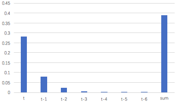
我们就可以看到，从上图的t-3时刻开始，梯度已经几乎减少到0了。那么，从这个时刻开始再往之前走，得到的梯度（几乎为零）就不会对最终的梯度值有任何贡献，这就相当于无论t-3时刻之前的网络状态h是什么，在训练中都不会对权重数组W的更新产生影响，也就是网络事实上已经忽略了t-3时刻之前的状态。这就是原始RNN无法处理长距离依赖的原因。

既然找到了问题的原因，那么我们就能解决它。从问题的定位到解决，科学家们大概花了7、8年时间。终于有一天，Hochreiter和Schmidhuber两位科学家发明出长短时记忆网络，一举解决这个问题。

其实，长短时记忆网络的思路比较简单。原始RNN的隐藏层只有一个状态，即h，它对于短期的输入非常敏感。那么，假如我们再增加一个状态，即c，让它来保存长期的状态，那么问题不就解决了么？如下图所示：

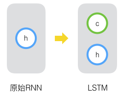
新增加的状态c，称为单元状态(cell state)。我们把上图按照时间维度展开：

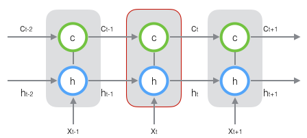
上图仅仅是一个示意图，我们可以看出，在t时刻，LSTM的输入有三个：当前时刻网络的输入值${\mathbf{x}}_t$、上一时刻LSTM的输出值${\mathbf{h}}_{t-1}$、以及上一时刻的单元状态${\mathbf{c}}_{t-1}$；LSTM的输出有两个：当前时刻LSTM输出值${\mathbf{h}}_t$、和当前时刻的单元状态${\mathbf{c}}_t$。注意$\mathbf{x}、\mathbf{h}、\mathbf{c}$都是向量。

LSTM的关键，就是怎样控制长期状态$c$。在这里，LSTM的思路是使用三个控制开关。第一个开关，负责控制继续保存长期状态$c$；第二个开关，负责控制把即时状态输入到长期状态$c$；第三个开关，负责控制是否把长期状态$c$作为当前的LSTM的输出。三个开关的作用如下图所示：

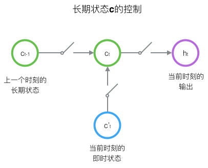
接下来，我们要描述一下，输出h和单元状态c的具体计算方法。

二、长短时记忆网络的前向计算

前面描述的开关是怎样在算法中实现的呢？这就用到了门（gate）的概念。门实际上就是一层全连接层，它的输入是一个向量，输出是一个0到1之间的实数向量。假设$W$是门的权重向量，$\mathbf{b}$是偏置项，那么门可以表示为：$$g(x)=\sigma (W\mathbf{x}+\mathbf{b})$$门的使用，就是用门的输出向量按元素乘以我们需要控制的那个向量。因为门的输出是0到1之间的实数向量，那么，当门输出为0时，任何向量与之相乘都会得到0向量，这就相当于啥都不能通过；输出为1时，任何向量与之相乘都不会有任何改变，这就相当于啥都可以通过。因为$\sigma$（也就是sigmoid函数）的值域是(0,1)，所以门的状态都是半开半闭的。

LSTM用两个门来控制单元状态$c$的内容，一个是遗忘门（forget gate），它决定了上一时刻的单元状态${\mathbf{c}}_{t-1}$有多少保留到当前时刻${\mathbf{c}}_t$；另一个是输入门（input gate），它决定了当前时刻网络的输入${\mathbf{x}}_t$有多少保存到单元状态${\mathbf{c}}_t$。LSTM用输出门（output gate）来控制单元状态${\mathbf{c}}_t$有多少输出到LSTM的当前输出值${\mathbf{h}}_t$。

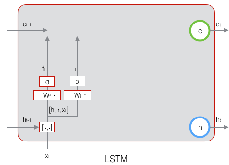
我们先来看一下遗忘门：$${\mathbf{f}}_t=\sigma (W_f\cdot [{\mathbf{h}}_{t-1},{\mathbf{x}}_t]+{\mathbf{b}}_f)(式1)$$上式中，$W_f$是遗忘门的权重矩阵，$[{\mathbf{h}}_{t-1},{\mathbf{x}}_t]$表示把两个向量连接成一个更长的向量，${\mathbf{b}}_f$是遗忘门的偏置项，$\sigma$是sigmoid函数。如果输入的维度是$d_x$，隐藏层的维度是$d_h$，单元状态的维度是$d_c$（通常$d_c=d_h$），则遗忘门的权重矩阵$W_f$维度是$d_c\times (d_h+d_x)$。事实上，权重矩阵$W_f$都是两个矩阵拼接而成的：一个是$W_{fh}$，它对应着输入项${\mathbf{h}}_{t-1}$，其维度为$d_c\times d_h$；一个是$W_{fx}$，它对应着输入项${\mathbf{x}}_t$，其维度为$d_c\times d_x$。$W_f$可以写为：$$[W_f]\left[\begin{array}{c}{\mathbf{h}}_{t-1}\\ {\mathbf{x}}_t\end{array}\right]=\left[\begin{array}{c}{W}_{fh}{W}_{fx}\end{array}\right]\left[\begin{array}{c}{\mathbf{h}}_{t-1}\\ {\mathbf{x}}_t\end{array}\right]$$$$=W_{fh}{\mathbf{h}}_{t-1}+W_{fx}{\mathbf{x}}_t$$下图显示了遗忘门的计算：

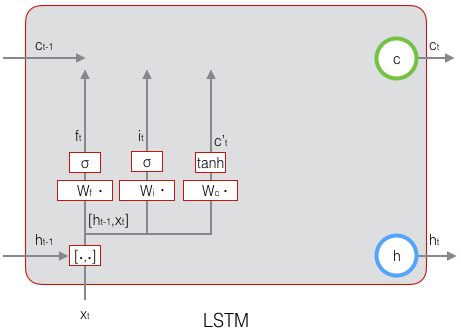
接下来看看输入门：
$${\mathbf{i}}_t=\sigma (W_i\cdot [{\mathbf{h}}_{t-1},{\mathbf{x}}_t]+{\mathbf{b}}_i)(式2)$$上式中，$W_i$是输入门的权重矩阵，${\mathbf{b}}_i$是输入门的偏置项。下图表示了输入门的计算：

接下来，我们计算用于描述当前输入的单元状态${\tilde{\mathbf{c}}}_t$，它是根据上一次的输出和本次输入来计算的：$${\tilde{\mathbf{c}}}_t=tanh(W_c\cdot [{\mathbf{h}}_{t-1},{\mathbf{x}}_t]+{\mathbf{b}}_c)(式3)$$下图是${\tilde{\mathbf{c}}}_t$的计算：

现在，我们计算当前时刻的单元状态${\mathbf{c}}_t$。它是由上一次的单元状态${\mathbf{c}}_{t-1}$按元素乘以遗忘门$f_t$，再用当前输入的单元状态${\tilde{\mathbf{c}}}_t$按元素乘以输入门$i_t$，再将两个积加和产生的：$${\mathbf{c}}_t=f_t\circ {\mathbf{c}}_{-1}+i_t\circ {\tilde{\mathbf{c}}}_t(式4)$$符号$\circ$表示按元素乘。下图是${\mathbf{c}}_t$的计算：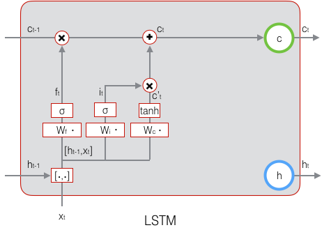
这样，我们就把LSTM关于当前的记忆${\tilde{\mathbf{c}}}_t$和长期的记忆${\mathbf{c}}_{t-1}$组合在一起，形成了新的单元状态${\mathbf{c}}_t$。由于遗忘门的控制，它可以保存很久很久之前的信息，由于输入门的控制，它又可以避免当前无关紧要的内容进入记忆。下面，我们要看看输出门，它控制了长期记忆对当前输出的影响：$${\mathbf{o}}_t=\sigma (W_o\cdot [{\mathbf{h}}_{t-1},{\mathbf{x}}_t]+{\mathbf{b}}_o)(式5)$$下图表示输出门的计算：
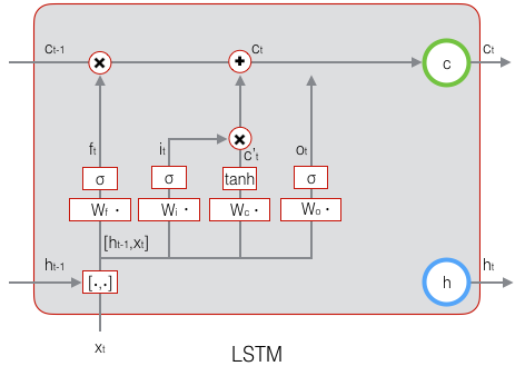
LSTM最终的输出，是由输出门和单元状态共同确定的：$${\mathbf{h}}_t={\mathbf{o}}_t\circ tanh({\mathbf{c}}_t)(式6)$$下图表示LSTM最终输出的计算：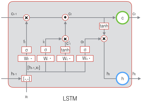
(式1)到(式6)就是LSTM前向计算的全部公式。至此，我们就把LSTM前向计算讲完了。

三、长短时记忆网络的训练

熟悉我们这个系列文章的同学都清楚，训练部分往往比前向计算部分复杂多了。LSTM的前向计算都这么复杂，那么，可想而知，它的训练算法一定是非常非常复杂的。现在只有做几次深呼吸，再一头扎进公式海洋吧。

LSTM训练算法框架

LSTM的训练算法仍然是反向传播算法，对于这个算法，我们已经非常熟悉了。主要有下面三个步骤：

1. 前向计算每个神经元的输出值，对于LSTM来说，即${\mathbf{f}}_t、{\mathbf{i}}_t、{\mathbf{c}}_t、{\mathbf{o}}_t、{\mathbf{h}}_t$五个向量的值。计算方法已经在上一节中描述过了。
2. 反向计算每个神经元的误差项$\delta$值。与循环神经网络一样，LSTM误差项的反向传播也是包括两个方向：一个是沿时间的反向传播，即从当前t时刻开始，计算每个时刻的误差项；一个是将误差项向上一层传播。
3. 根据相应的误差项，计算每个权重的梯度。

关于公式和符号的说明

首先，我们对推导中用到的一些公式、符号做一下必要的说明。

接下来的推导中，我们设定gate的激活函数为sigmoid函数，输出的激活函数为tanh函数。他们的导数分别为：
$$\sigma (z)=y=\frac{1}{1+e^{-z}}$$$${\sigma }^{\prime }(z)=y(1-y)$$$$tanh(z)=y=\frac{e^z-e^{-z}}{e^z+e^{-z}}$$$$tan{h}^{\prime }(z)=1-y^2$$从上面可以看出，sigmoid和tanh函数的导数都是原函数的函数。这样，我们一旦计算原函数的值，就可以用它来计算出导数的值。

LSTM需要学习的参数共有8组，分别是：遗忘门的权重矩阵$W_f$和偏置项${\mathbf{b}}_f$、输入门的权重矩阵$W_i$和偏置项${\mathbf{b}}_i$、输出门的权重矩阵$W_o$和偏置项${\mathbf{b}}_o$，以及计算单元状态的权重矩阵$W_c$和偏置项${\mathbf{b}}_c$。因为权重矩阵的两部分在反向传播中使用不同的公式，因此在后续的推导中，权重矩阵$W_f、W_i、W_o、W_c$都将被写为分开的两个矩阵：$W_{fh}、W_{fx}、W_{ih}、W_{ix}、W_{oh}、W_{ox}、W_{ch}、W_{cx}$。

我们解释一下按元素乘$\circ$符号。当$\circ$作用于两个向量时，运算如下：$$a\circ b=\left[\begin{array}{c}{a}_1\\ a_2\\ a_3\\ ...\\ a_n\end{array}\right]\circ \left[\begin{array}{c}{b}_1\\ b_2\\ b_3\\ ...\\ b_n\end{array}\right]=\left[\begin{array}{c}{a}_1{b}_1\\ a_2{b}_2\\ a_3{b}_3\\ ...\\ a_n{b}_n\end{array}\right]$$当$\circ$作用于一个向量和一个矩阵时，运算如下：$$a\circ X=\left[\begin{array}{c}{a}_1\\ a_2\\ a_3\\ ...\\ a_n\end{array}\right]\circ \left[\begin{array}{c}{x}_{11}{x}_{12}...x_{1n}\\ x_{21}{x}_{22}...x_{2n}\\ x_{31}{x}_{32}...x_{3n}\\ ...\\ x_{n1}{x}_{n2}...x_{nn}\end{array}\right]$$$$=\left[\begin{array}{c}{a}_1{x}_{11}{a}_1{x}_{12}...a_1{x}_{1n}\\ a_2{x}_{21}{a}_2{x}_{22}...a_2{x}_{2n}\\ a_3{x}_{31}{a}_3{x}_{32}...a_3{x}_{3n}\\ ...\\ a_n{x}_{n1}{a}_n{x}_{n2}...a_n{x}_{nn}\end{array}\right]$$当$\circ$作用于两个矩阵时，两个矩阵对应位置的元素相乘。按元素乘可以在某些情况下简化矩阵和向量运算。例如，当一个对角矩阵右乘一个矩阵时，相当于用对角矩阵的对角线组成的向量按元素乘那个矩阵：$$diag[a]X=a\circ X$$当一个行向量右乘一个对角矩阵时，相当于这个行向量按元素乘那个矩阵对角线组成的向量：$$a^{T}diag[b]=a\circ b$$上面这两点，在我们后续推导中会多次用到。

在t时刻，LSTM的输出值为${\mathbf{h}}_t$。我们定义t时刻的误差项${\delta }_t$为：$${\delta }_t\stackrel{def}{=}\frac{\partial E}{\partial {\mathbf{h}}_t}$$注意，和前面几篇文章不同，我们这里假设误差项是损失函数对输出值的导数，而不是对加权输入$ne{t}_t^l$的导数。因为LSTM有四个加权输入，分别对应${\mathbf{f}}_t、{\mathbf{i}}_t、{\mathbf{c}}_t、{\mathbf{o}}_t$，我们希望往上一层传递一个误差项而不是四个。但我们仍然需要定义出这四个加权输入，以及他们对应的误差项。$$ne{t}_{f,t}=W_f[{\mathbf{h}}_{t-1},{\mathbf{x}}_t]+{\mathbf{b}}_f$$$$=W_{fh}{\mathbf{h}}_{t-1}+W_{fx}{\mathbf{x}}_t+{\mathbf{b}}_f$$$$ne{t}_{i,t}=W_i[{\mathbf{h}}_{t-1},{\mathbf{x}}_t]+{\mathbf{b}}_i$$$$=W_{ih}{\mathbf{h}}_{t-1}+W_{ix}{\mathbf{x}}_t+{\mathbf{b}}_i$$$$ne{t}_{\tilde{c},t}=W_c[{\mathbf{h}}_{t-1},{\mathbf{x}}_t]+{\mathbf{b}}_c$$$$=W_{ch}{\mathbf{h}}_{t-1}+W_{cx}{\mathbf{x}}_t+{\mathbf{b}}_c$$$$ne{t}_{o,t}=W_o[{\mathbf{h}}_{t-1},{\mathbf{x}}_t]+{\mathbf{b}}_o$$$$=W_{oh}{\mathbf{h}}_{t-1}+W_{ox}{\mathbf{x}}_t+{\mathbf{b}}_o$$$${\delta }_{f,t}\stackrel{def}{=}\frac{\partial E}{\partial ne{t}_{f,t}}$$$${\delta }_{i,t}\stackrel{def}{=}\frac{\partial E}{\partial ne{t}_{i,t}}$$$${\delta }_{\tilde{c},t}\stackrel{def}{=}\frac{\partial E}{\partial ne{t}_{\tilde{c},t}}$$$${\delta }_{o,t}\stackrel{def}{=}\frac{\partial E}{\partial ne{t}_{o,t}}$$

误差项沿时间的反向传递

沿时间反向传递误差项，就是要计算出t-1时刻的误差项${\delta }_{t-1}$。$${\delta }_{t-1}^T=\frac{\partial E}{\partial {\mathbf{h}}_{t-1}}$$$$=\frac{\partial E}{\partial {\mathbf{h}}_t}\frac{\partial {\mathbf{h}}_t}{\partial {\mathbf{h}}_{t-1}}$$$$={\delta }_t^T\frac{\partial {\mathbf{h}}_t}{\partial {\mathbf{h}}_{t-1}}$$我们知道，$\frac{\partial {\mathbf{h}}_t}{\partial {\mathbf{h}}_{t-1}}$是一个Jacobian矩阵。如果隐藏层h的维度是N的话，那么它就是一个$N\times N$矩阵。为了求出它，我们列出${\mathbf{h}}_t$的计算公式，即前面的(式6)和(式4)：$${\mathbf{h}}_t={\mathbf{o}}_t\circ tanh({\mathbf{c}}_t)$$$${\mathbf{c}}_t={\mathbf{f}}_t\circ {\mathbf{c}}_{t-1}+{\mathbf{i}}_t\circ {\tilde{\mathbf{c}}}_t$$显然，${\mathbf{o}}_t、{\mathbf{f}}_t、{\mathbf{i}}_t、{\tilde{\mathbf{c}}}_t$都是${\mathbf{h}}_{t-1}$的函数，那么，利用全导数公式可得：
$${\delta }_t^T\frac{\partial {\mathbf{h}}_{\mathbf{t}}}{\partial {\mathbf{h}}_{\mathbf{t}-1}}={\delta }_t^T\frac{\partial {\mathbf{h}}_{\mathbf{t}}}{\partial {\mathbf{o}}_t}\frac{\partial {\mathbf{o}}_t}{\partial {\mathbf{n}\mathbf{e}\mathbf{t}}_{o,t}}\frac{\partial {\mathbf{n}\mathbf{e}\mathbf{t}}_{o,t}}{\partial {\mathbf{h}}_{\mathbf{t}-1}}+{\delta }_t^T\frac{\partial {\mathbf{h}}_{\mathbf{t}}}{\partial {\mathbf{c}}_t}\frac{\partial {\mathbf{c}}_t}{\partial {\mathbf{f}}_{\mathbf{t}}}\frac{\partial {\mathbf{f}}_t}{\partial {\mathbf{n}\mathbf{e}\mathbf{t}}_{f,t}}\frac{\partial {\mathbf{n}\mathbf{e}\mathbf{t}}_{f,t}}{\partial {\mathbf{h}}_{\mathbf{t}-1}}+{\delta }_t^T\frac{\partial {\mathbf{h}}_{\mathbf{t}}}{\partial {\mathbf{c}}_t}\frac{\partial {\mathbf{c}}_t}{\partial {\mathbf{i}}_{\mathbf{t}}}\frac{\partial {\mathbf{i}}_t}{\partial {\mathbf{n}\mathbf{e}\mathbf{t}}_{i,t}}\frac{\partial {\mathbf{n}\mathbf{e}\mathbf{t}}_{i,t}}{\partial {\mathbf{h}}_{\mathbf{t}-1}}+{\delta }_t^T\frac{\partial {\mathbf{h}}_{\mathbf{t}}}{\partial {\mathbf{c}}_t}\frac{\partial {\mathbf{c}}_t}{\partial {\tilde{\mathbf{c}}}_t}\frac{\partial {\tilde{\mathbf{c}}}_t}{\partial {\mathbf{n}\mathbf{e}\mathbf{t}}_{\tilde{c},t}}\frac{\partial {\mathbf{n}\mathbf{e}\mathbf{t}}_{\tilde{c},t}}{\partial {\mathbf{h}}_{\mathbf{t}-1}}$$$$={\delta }_{o,t}^T\frac{\partial {\mathbf{n}\mathbf{e}\mathbf{t}}_{o,t}}{\partial {\mathbf{h}}_{\mathbf{t}-1}}+{\delta }_{f,t}^T\frac{\partial {\mathbf{n}\mathbf{e}\mathbf{t}}_{f,t}}{\partial {\mathbf{h}}_{\mathbf{t}-1}}+{\delta }_{i,t}^T\frac{\partial {\mathbf{n}\mathbf{e}\mathbf{t}}_{i,t}}{\partial {\mathbf{h}}_{\mathbf{t}-1}}+{\delta }_{\tilde{c},t}^T\frac{\partial {\mathbf{n}\mathbf{e}\mathbf{t}}_{\tilde{c},t}}{\partial {\mathbf{h}}_{\mathbf{t}-1}}(式7)$$下面，我们要把(式7)中的每个偏导数都求出来。根据(式6)，我们可以求出：$$\frac{\partial {\mathbf{h}}_{\mathbf{t}}}{\partial {\mathbf{o}}_t}=diag[\tanh ({\mathbf{c}}_t)]$$$$\frac{\partial {\mathbf{h}}_{\mathbf{t}}}{\partial {\mathbf{c}}_t}=diag[{\mathbf{o}}_t\circ (1-\tanh ({\mathbf{c}}_t{)}^2)]$$根据(式4)，我们可以求出：$$\frac{\partial {\mathbf{c}}_t}{\partial {\mathbf{f}}_{\mathbf{t}}}=diag[{\mathbf{c}}_{t-1}]$$$$\frac{\partial {\mathbf{c}}_t}{\partial {\mathbf{i}}_{\mathbf{t}}}=diag[{\tilde{\mathbf{c}}}_t]$$$$\frac{\partial {\mathbf{c}}_t}{\partial {\tilde{\mathbf{c}}}_{\mathbf{t}}}=diag[{\mathbf{i}}_t]$$因为：$${\mathbf{o}}_t=\sigma ({\mathbf{n}\mathbf{e}\mathbf{t}}_{o,t})$$$${\mathbf{n}\mathbf{e}\mathbf{t}}_{o,t}=W_{oh}{\mathbf{h}}_{t-1}+W_{ox}{\mathbf{x}}_t+{\mathbf{b}}_o$$$${\mathbf{f}}_t=\sigma ({\mathbf{n}\mathbf{e}\mathbf{t}}_{f,t})$$$${\mathbf{n}\mathbf{e}\mathbf{t}}_{f,t}=W_{fh}{\mathbf{h}}_{t-1}+W_{fx}{\mathbf{x}}_t+{\mathbf{b}}_f$$$${\mathbf{i}}_t=\sigma ({\mathbf{n}\mathbf{e}\mathbf{t}}_{i,t})$$$${\mathbf{n}\mathbf{e}\mathbf{t}}_{i,t}=W_{ih}{\mathbf{h}}_{t-1}+W_{ix}{\mathbf{x}}_t+{\mathbf{b}}_i$$$${\tilde{\mathbf{c}}}_t=\tanh ({\mathbf{n}\mathbf{e}\mathbf{t}}_{\tilde{c},t})$$$${\mathbf{n}\mathbf{e}\mathbf{t}}_{\tilde{c},t}=W_{ch}{\mathbf{h}}_{t-1}+W_{cx}{\mathbf{x}}_t+{\mathbf{b}}_c$$我们很容易得出：$$\frac{\partial {\mathbf{o}}_t}{\partial {\mathbf{n}\mathbf{e}\mathbf{t}}_{o,t}}=diag[{\mathbf{o}}_t\circ (1-{\mathbf{o}}_t)]$$$$\frac{\partial {\mathbf{n}\mathbf{e}\mathbf{t}}_{o,t}}{\partial {\mathbf{h}}_{\mathbf{t}-1}}=W_{oh}$$$$\frac{\partial {\mathbf{f}}_t}{\partial {\mathbf{n}\mathbf{e}\mathbf{t}}_{f,t}}=diag[{\mathbf{f}}_t\circ (1-{\mathbf{f}}_t)]$$$$\frac{\partial {\mathbf{n}\mathbf{e}\mathbf{t}}_{f,t}}{\partial {\mathbf{h}}_{t-1}}=W_{fh}$$$$\frac{\partial {\mathbf{i}}_t}{\partial {\mathbf{n}\mathbf{e}\mathbf{t}}_{i,t}}=diag[{\mathbf{i}}_t\circ (1-{\mathbf{i}}_t)]$$$$\frac{\partial {\mathbf{n}\mathbf{e}\mathbf{t}}_{i,t}}{\partial {\mathbf{h}}_{t-1}}=W_{ih}$$$$\frac{\partial {\tilde{\mathbf{c}}}_t}{\partial {\mathbf{n}\mathbf{e}\mathbf{t}}_{\tilde{c},t}}=diag[1-{\tilde{\mathbf{c}}}_t^2]$$$$\frac{\partial {\mathbf{n}\mathbf{e}\mathbf{t}}_{\tilde{c},t}}{\partial {\mathbf{h}}_{t-1}}=W_{ch}$$将上述偏导数带入到（式7），我们得到：$${\delta }_{t-1}={\delta }_{o,t}^T\frac{\partial {\mathbf{n}\mathbf{e}\mathbf{t}}_{o,t}}{\partial {\mathbf{h}}_{\mathbf{t}-1}}+{\delta }_{f,t}^T\frac{\partial {\mathbf{n}\mathbf{e}\mathbf{t}}_{f,t}}{\partial {\mathbf{h}}_{\mathbf{t}-1}}+{\delta }_{i,t}^T\frac{\partial {\mathbf{n}\mathbf{e}\mathbf{t}}_{i,t}}{\partial {\mathbf{h}}_{\mathbf{t}-1}}+{\delta }_{\tilde{c},t}^T\frac{\partial {\mathbf{n}\mathbf{e}\mathbf{t}}_{\tilde{c},t}}{\partial {\mathbf{h}}_{\mathbf{t}-1}}$$$$={\delta }_{o,t}^T{W}_{oh}+{\delta }_{f,t}^T{W}_{fh}+{\delta }_{i,t}^T{W}_{ih}+{\delta }_{\tilde{c},t}^T{W}_{ch}(式8)$$根据${\delta }_{o,t}、{\delta }_{f,t}、{\delta }_{i,t}、{\delta }_{\tilde{c},t}$的定义，可知：$${\delta }_{o,t}^T={\delta }_t^T\circ \tanh ({\mathbf{c}}_t)\circ {\mathbf{o}}_t\circ (1-{\mathbf{o}}_t)(式9)$$$${\delta }_{f,t}^T={\delta }_t^T\circ {\mathbf{o}}_t\circ (1-\tanh ({\mathbf{c}}_t{)}^2)\circ {\mathbf{c}}_{t-1}\circ {\mathbf{f}}_t\circ (1-{\mathbf{f}}_t)(式10)$$$${\delta }_{i,t}^T={\delta }_t^T\circ {\mathbf{o}}_t\circ (1-\tanh ({\mathbf{c}}_t{)}^2)\circ {\tilde{\mathbf{c}}}_t\circ {\mathbf{i}}_t\circ (1-{\mathbf{i}}_t)(式11)$$$${\delta }_{\tilde{c},t}^T={\delta }_t^T\circ {\mathbf{o}}_t\circ (1-\tanh ({\mathbf{c}}_t{)}^2)\circ {\mathbf{i}}_t\circ (1-{\tilde{\mathbf{c}}}^2)(式12)$$(式8)到(式12)就是将误差沿时间反向传播一个时刻的公式。有了它，我们可以写出将误差项向前传递到任意k时刻的公式：$${\delta }_k^T=\prod _{j=k}^{t-1}{\delta }_{o,j}^T{W}_{oh}+{\delta }_{f,j}^T{W}_{fh}+{\delta }_{i,j}^T{W}_{ih}+{\delta }_{\tilde{c},j}^T{W}_{ch}(式13)$$

将误差项传递到上一层

我们假设当前为第$l$层，定义$l-1$层的误差项是误差函数对$l-1$层加权输入的导数，即：$${\delta }_t^{l-1}\stackrel{def}{=}\frac{\partial E}{{\mathbf{n}\mathbf{e}\mathbf{t}}_t^{l-1}}$$本次LSTM的输入$x_t$由下面的公式计算：$${\mathbf{x}}_t^l=f^{l-1}({\mathbf{n}\mathbf{e}\mathbf{t}}_t^{l-1})$$上式中，$f^{l-1}$表示第$l-1$层的激活函数。

因为${\mathbf{n}\mathbf{e}\mathbf{t}}_{f,t}^l、{\mathbf{n}\mathbf{e}\mathbf{t}}_{i,t}^l、{\mathbf{n}\mathbf{e}\mathbf{t}}_{\tilde{c},t}^l、{\mathbf{n}\mathbf{e}\mathbf{t}}_{o,t}^l$都是$x_t$的函数，$x_t$又是$ne{t}_t^{l-1}$的函数，因此，要求出$E$对$ne{t}_t^{l-1}$的导数，就需要使用全导数公式：$$\frac{\partial E}{\partial {\mathbf{n}\mathbf{e}\mathbf{t}}_t^{l-1}}=\frac{\partial E}{\partial {\mathbf{n}\mathbf{e}\mathbf{t}}_{\mathbf{f},\mathbf{t}}^{\mathbf{l}}}\frac{\partial {\mathbf{n}\mathbf{e}\mathbf{t}}_{\mathbf{f},\mathbf{t}}^{\mathbf{l}}}{\partial {\mathbf{x}}_t^l}\frac{\partial {\mathbf{x}}_t^l}{\partial {\mathbf{n}\mathbf{e}\mathbf{t}}_{\mathbf{t}}^{\mathbf{l}-1}}+\frac{\partial E}{\partial {\mathbf{n}\mathbf{e}\mathbf{t}}_{\mathbf{i},\mathbf{t}}^{\mathbf{l}}}\frac{\partial {\mathbf{n}\mathbf{e}\mathbf{t}}_{\mathbf{i},\mathbf{t}}^{\mathbf{l}}}{\partial {\mathbf{x}}_t^l}\frac{\partial {\mathbf{x}}_t^l}{\partial {\mathbf{n}\mathbf{e}\mathbf{t}}_{\mathbf{t}}^{\mathbf{l}-1}}+\frac{\partial E}{\partial {\mathbf{n}\mathbf{e}\mathbf{t}}_{\tilde{\mathbf{c}},\mathbf{t}}^{\mathbf{l}}}\frac{\partial {\mathbf{n}\mathbf{e}\mathbf{t}}_{\tilde{\mathbf{c}},\mathbf{t}}^{\mathbf{l}}}{\partial {\mathbf{x}}_t^l}\frac{\partial {\mathbf{x}}_t^l}{\partial {\mathbf{n}\mathbf{e}\mathbf{t}}_{\mathbf{t}}^{\mathbf{l}-1}}+\frac{\partial E}{\partial {\mathbf{n}\mathbf{e}\mathbf{t}}_{\mathbf{o},\mathbf{t}}^{\mathbf{l}}}\frac{\partial {\mathbf{n}\mathbf{e}\mathbf{t}}_{\mathbf{o},\mathbf{t}}^{\mathbf{l}}}{\partial {\mathbf{x}}_t^l}\frac{\partial {\mathbf{x}}_t^l}{\partial {\mathbf{n}\mathbf{e}\mathbf{t}}_{\mathbf{t}}^{\mathbf{l}-1}}$$$$={\delta }_{f,t}^T{W}_{fx}\circ f^{\prime }({\mathbf{n}\mathbf{e}\mathbf{t}}_t^{l-1})+{\delta }_{i,t}^T{W}_{ix}\circ f^{\prime }({\mathbf{n}\mathbf{e}\mathbf{t}}_t^{l-1})+{\delta }_{\tilde{c},t}^T{W}_{cx}\circ f^{\prime }({\mathbf{n}\mathbf{e}\mathbf{t}}_t^{l-1})+{\delta }_{o,t}^T{W}_{ox}\circ f^{\prime }({\mathbf{n}\mathbf{e}\mathbf{t}}_t^{l-1})$$$$=({\delta }_{f,t}^T{W}_{fx}+{\delta }_{i,t}^T{W}_{ix}+{\delta }_{\tilde{c},t}^T{W}_{cx}+{\delta }_{o,t}^T{W}_{ox})\circ f^{\prime }({\mathbf{n}\mathbf{e}\mathbf{t}}_t^{l-1})(式14)$$(式14)就是将误差传递到上一层的公式。

权重梯度的计算

对于$W_{ft}、W_{ih}、W_{ch}、W_{oh}$的权重梯度，我们知道它的梯度是各个时刻梯度之和（证明过程请参考文章《深度学习之循环神经网络(RNN)》），我们首先求出它们在t时刻的梯度，然后再求出他们最终的梯度。

我们已经求得了误差项${\delta }_{o,t}、{\delta }_{f,t}、{\delta }_{i,t}、{\delta }_{\tilde{c},t}$，很容易求出t时刻的$W_{oh}、W_{ih}、W_{fh}、W_{ch}$：$$\frac{\partial E}{\partial W_{oh,t}}=\frac{\partial E}{\partial {\mathbf{n}\mathbf{e}\mathbf{t}}_{o,t}}\frac{\partial {\mathbf{n}\mathbf{e}\mathbf{t}}_{o,t}}{\partial W_{oh,t}}$$$$={\delta }_{o,t}{\mathbf{h}}_{t-1}^T$$$$\frac{\partial E}{\partial W_{fh,t}}=\frac{\partial E}{\partial {\mathbf{n}\mathbf{e}\mathbf{t}}_{f,t}}\frac{\partial {\mathbf{n}\mathbf{e}\mathbf{t}}_{f,t}}{\partial W_{fh,t}}$$$$={\delta }_{f,t}{\mathbf{h}}_{t-1}^T$$$$\frac{\partial E}{\partial W_{ih,t}}=\frac{\partial E}{\partial {\mathbf{n}\mathbf{e}\mathbf{t}}_{i,t}}\frac{\partial {\mathbf{n}\mathbf{e}\mathbf{t}}_{i,t}}{\partial W_{ih,t}}$$$$={\delta }_{i,t}{\mathbf{h}}_{t-1}^T$$$$\frac{\partial E}{\partial W_{ch,t}}=\frac{\partial E}{\partial {\mathbf{n}\mathbf{e}\mathbf{t}}_{\tilde{c},t}}\frac{\partial {\mathbf{n}\mathbf{e}\mathbf{t}}_{\tilde{c},t}}{\partial W_{ch,t}}$$$$={\delta }_{\tilde{c},t}{\mathbf{h}}_{t-1}^T$$将各个时刻的梯度加在一起，就能得到最终的梯度：$$\frac{\partial E}{\partial W_{oh}}=\sum _{j=1}^t{\delta }_{o,j}{\mathbf{h}}_{j-1}^T$$$$\frac{\partial E}{\partial W_{fh}}=\sum _{j=1}^t{\delta }_{f,j}{\mathbf{h}}_{j-1}^T$$$$\frac{\partial E}{\partial W_{ih}}=\sum _{j=1}^t{\delta }_{i,j}{\mathbf{h}}_{j-1}^T$$$$\frac{\partial E}{\partial W_{ch}}=\sum _{j=1}^t{\delta }_{\tilde{c},j}{\mathbf{h}}_{j-1}^T$$对于偏置项${\mathbf{b}}_f、{\mathbf{b}}_i、{\mathbf{b}}_c、{\mathbf{b}}_o$的梯度，也是将各个时刻的梯度加在一起。下面是各个时刻的偏置项梯度：$$\frac{\partial E}{\partial {\mathbf{b}}_{o,t}}=\frac{\partial E}{\partial {\mathbf{n}\mathbf{e}\mathbf{t}}_{o,t}}\frac{\partial {\mathbf{n}\mathbf{e}\mathbf{t}}_{o,t}}{\partial {\mathbf{b}}_{o,t}}$$$$={\delta }_{o,t}$$$$\frac{\partial E}{\partial {\mathbf{b}}_{f,t}}=\frac{\partial E}{\partial {\mathbf{n}\mathbf{e}\mathbf{t}}_{f,t}}\frac{\partial {\mathbf{n}\mathbf{e}\mathbf{t}}_{f,t}}{\partial {\mathbf{b}}_{f,t}}$$$$={\delta }_{f,t}$$$$\frac{\partial E}{\partial {\mathbf{b}}_{i,t}}=\frac{\partial E}{\partial {\mathbf{n}\mathbf{e}\mathbf{t}}_{i,t}}\frac{\partial {\mathbf{n}\mathbf{e}\mathbf{t}}_{i,t}}{\partial {\mathbf{b}}_{i,t}}$$$$={\delta }_{i,t}$$$$\frac{\partial E}{\partial {\mathbf{b}}_{c,t}}=\frac{\partial E}{\partial {\mathbf{n}\mathbf{e}\mathbf{t}}_{\tilde{c},t}}\frac{\partial {\mathbf{n}\mathbf{e}\mathbf{t}}_{\tilde{c},t}}{\partial {\mathbf{b}}_{c,t}}$$$$={\delta }_{\tilde{c},t}$$下面是最终的偏置项梯度，即将各个时刻的偏置项梯度加在一起：$$\frac{\partial E}{\partial {\mathbf{b}}_o}=\sum _{j=1}^t{\delta }_{o,j}$$$$\frac{\partial E}{\partial {\mathbf{b}}_i}=\sum _{j=1}^t{\delta }_{i,j}$$$$\frac{\partial E}{\partial {\mathbf{b}}_f}=\sum _{j=1}^t{\delta }_{f,j}$$$$\frac{\partial E}{\partial {\mathbf{b}}_c}=\sum _{j=1}^t{\delta }_{\tilde{c},j}$$对于$W_{fx}、W_{ix}、W_{cx}、W_{ox}$的权重梯度，只需要根据相应的误差项直接计算即可：$$\frac{\partial E}{\partial W_{ox}}=\frac{\partial E}{\partial {\mathbf{n}\mathbf{e}\mathbf{t}}_{o,t}}\frac{\partial {\mathbf{n}\mathbf{e}\mathbf{t}}_{o,t}}{\partial W_{ox}}$$$$={\delta }_{o,t}{\mathbf{x}}_t^T$$$$\frac{\partial E}{\partial W_{fx}}=\frac{\partial E}{\partial {\mathbf{n}\mathbf{e}\mathbf{t}}_{f,t}}\frac{\partial {\mathbf{n}\mathbf{e}\mathbf{t}}_{f,t}}{\partial W_{fx}}$$$$={\delta }_{f,t}{\mathbf{x}}_t^T$$$$\frac{\partial E}{\partial W_{ix}}=\frac{\partial E}{\partial {\mathbf{n}\mathbf{e}\mathbf{t}}_{i,t}}\frac{\partial {\mathbf{n}\mathbf{e}\mathbf{t}}_{i,t}}{\partial W_{ix}}$$$$={\delta }_{i,t}{\mathbf{x}}_t^T$$$$\frac{\partial E}{\partial W_{cx}}=\frac{\partial E}{\partial {\mathbf{n}\mathbf{e}\mathbf{t}}_{\tilde{c},t}}\frac{\partial {\mathbf{n}\mathbf{e}\mathbf{t}}_{\tilde{c},t}}{\partial W_{cx}}$$$$={\delta }_{\tilde{c},t}{\mathbf{x}}_t^T$$
以上就是LSTM的训练算法的全部公式。因为这里面存在很多重复的模式，仔细看看，会发觉并不是太复杂。

当然，LSTM存在着相当多的变体，读者可以在互联网上找到很多资料。因为大家已经熟悉了基本LSTM的算法，因此理解这些变体比较容易，因此本文就不再赘述了。

四、GRU

前面我们讲了一种普通的LSTM，事实上LSTM存在很多变体，许多论文中的LSTM都或多或少的不太一样。在众多的LSTM变体中，**GRU (Gated Recurrent Unit)**也许是最成功的一种。它对LSTM做了很多简化，同时却保持着和LSTM相同的效果。因此，GRU最近变得越来越流行。

GRU对LSTM做了两个大改动：

1. 将输入门、遗忘门、输出门变为两个门：更新门（Update Gate）${\mathbf{z}}_t$和重置门（Reset Gate）${\mathbf{r}}_t$。
2. 将单元状态与输出合并为一个状态：$\mathbf{h}$。

GRU的前向计算公式为：$${\mathbf{z}}_t=\sigma (W_z\cdot [{\mathbf{h}}_{t-1},{\mathbf{x}}_t])$$$${\mathbf{r}}_t=\sigma (W_r\cdot [{\mathbf{h}}_{t-1},{\mathbf{x}}_t])$$$${\tilde{\mathbf{h}}}_t=\tanh (W\cdot [{\mathbf{r}}_t\circ {\mathbf{h}}_{t-1},{\mathbf{x}}_t])$$$$\mathbf{h}=(1-{\mathbf{z}}_t)\circ {\mathbf{h}}_{t-1}+{\mathbf{z}}_t\circ {\tilde{\mathbf{h}}}_t$$下图是GRU的示意图：
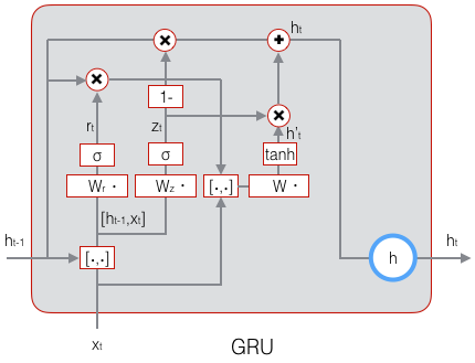
GRU的训练算法比LSTM简单一些，留给读者自行推导，本文就不再赘述了。

五、小结

至此，LSTM——也许是结构最复杂的一类神经网络——就讲完了，相信拿下前几篇文章的读者们搞定这篇文章也不在话下吧！现在我们已经了解循环神经网络和它最流行的变体——LSTM，它们都可以用来处理序列。但是，有时候仅仅拥有处理序列的能力还不够，还需要处理比序列更为复杂的结构（比如树结构），这时候就需要用到另外一类网络：递归神经网络(Recursive Neural Network)，巧合的是，它的缩写也是RNN。