python数据分析—二手车价格预测

目录

1.导入模块

2.数据的读取和初步处理

3.查补缺失值

4.模型初始化和数据准备

5，总结

---

1.导入模块

1.1环境准备：首先，确保你已经安装了xgboost。如果没有，可以通过pip来安装：

pip install xgboost

1.2导入必要的模块

import numpy as np
import pandas as pd
import matplotlib.pyplot as plt
import seaborn as sns
import warnings
from sklearn.ensemble import RandomForestRegressor, GradientBoostingRegressor
from xgboost import XGBRegressor
from sklearn.model_selection import cross_val_score, GridSearchCV 
pd.options.display.max_columns = None 
warnings.filterwarnings('ignore') 

2.数据的读取和初步处理

# 数据的读取和初步处理
df_train = pd.read_csv('used_car_train_20200313.csv', sep=' ')
df_test = pd.read_csv('used_car_testB_20200421.csv', sep=' ')
train = df_train.drop(['SaleID'], axis=1)
test = df_test.drop(['SaleID'], axis=1)

train.head()

test.head()

# 查看总览 - 训练集
train.info()

# 查看总览 - 测试集
test.info()

# 转换'-'
train['notRepairedDamage'] = train['notRepairedDamage'].replace('-', np.nan) 
test['notRepairedDamage'] = test['notRepairedDamage'].replace('-', np.nan)

# 转换数据类型
train['notRepairedDamage'] = train['notRepairedDamage'].astype('float64')
test['notRepairedDamage'] = test['notRepairedDamage'].astype('float64')

# 检查是否转换成功
train['notRepairedDamage'].unique(), test['notRepairedDamage'].unique()

# 查看数值统计描述 - 测试集
test.describe()

# 查看数值统计描述 - 训练集
train.describe()

train.drop(['seller'], axis=1, inplace=True)
test.drop(['seller'], axis=1, inplace=True)

train = train.drop(['offerType'], axis=1)
test = test.drop(['offerType'], axis=1)

# 有143个值不合法，需要用别的值替换
train[train['power'] > 600]['power'].count()

test[test['power'] > 600]['power'].count()

3.查补缺失值

# 查看训练集缺失值存在情况
train.isnull().sum()[train.isnull().sum() > 0]
# 查看测试集缺失值存在情况
test.isnull().sum()[test.isnull().sum() > 0]

train[train['model'].isnull()]

# model(车型编码)一般与brand, bodyType, gearbox, power有关，选择以上4个特征与该车相同的车辆的model，选择出现次数最多的值
train[(train['brand'] == 37) & 
      (train['bodyType'] == 6.0) & 
      (train['gearbox'] == 1.0) & 
      (train['power'] == 190)]['model'].value_counts()

# 用157.0填充缺失值
train.loc[38424, 'model'] = 157.0

train.loc[38424, :]

# 查看填充结果
train.info()

# 看缺失值数量
print(train['bodyType'].isnull().value_counts())
print('\n')
print(test['bodyType'].isnull().value_counts())

# 可见不同车身类型的汽车售价差别还是比较大的，故保留该特征，填充缺失值
# 看看车身类型数量分布
print(train['bodyType'].value_counts())
print('\n')
print(test['bodyType'].value_counts())

# 在两个数据集上，车身类型为0.0（豪华轿车）的汽车数量都是最多，所以用0.0来填充缺失值
train.loc[:, 'bodyType'] = train['bodyType'].map(lambda x: 0.0 if pd.isnull(x) else x)
test.loc[:, 'bodyType'] = test['bodyType'].map(lambda x: 0.0 if pd.isnull(x) else x)

# 看缺失值数量
print(train['fuelType'].isnull().value_counts())
print('\n')
print(test['fuelType'].isnull().value_counts())

# 猜想：燃油类型与车身类型相关，如豪华轿车更可能是汽油或电动， 而搅拌车大多是柴油
# 创建字典，保存不同bodyType下， fuelType的众数，并以此填充fuelTyp的缺失值
dict_enu_train, dict_enu_test = {}, {}
for i in [0.0, 1.0, 2.0, 3.0, 4.0, 5.0, 6.0, 7.0]:
    dict_enu_train[i] = train[train['bodyType'] == i]['fuelType'].mode()[0]
    dict_enu_test[i] = test[test['bodyType'] == i]['fuelType'].mode()[0]
    
# 发现dict_enu_train, dict_enu_test是一样的内容

# 开始填充fuelType缺失值
# 在含fuelType缺失值的条目中，将不同bodyType对应的index输出保存到一个字典中
dict_index_train, dict_index_test = {}, {}

for bodytype in [0.0, 1.0, 2.0, 3.0, 4.0, 5.0, 6.0, 7.0]:
    dict_index_train[bodytype] = train[(train['bodyType'] == bodytype) & (train['fuelType'].isnull())].index.tolist()
    dict_index_test[bodytype] = test[(test['bodyType'] == bodytype) & (test['fuelType'].isnull())].index.tolist()

# 分别对每个bodyTYpe所对应的index来填充fuelType列
for bt, ft in dict_enu_train.items():
#     train.loc[tuple(dict_index[bt]), :]['fuelType'] = ft  # 注意：链式索引 (chained indexing)很可能导致赋值失败！
    train.loc[dict_index_train[bt], 'fuelType'] = ft  # Pandas推荐使用这种方法来索引/赋值
    test.loc[dict_index_test[bt], 'fuelType'] = ft

# 看缺失值数量
print(train['gearbox'].isnull().value_counts())
print('\n')
print(test['gearbox'].isnull().value_counts())

# 可见变速箱类型的不同不会显著影响售价，删去测试集中带缺失值的行或许是可行的做法，但为避免样本量减少带来的过拟合，还是决定保留该特征并填充其缺失值
# 看看车身类型数量分布
print(train['gearbox'].value_counts())
print('\n')
print(test['gearbox'].value_counts())
test.info()

# 看缺失值数量
# 缺失值数量在两个数据集中的占比都不低
print(train['notRepairedDamage'].isnull().value_counts())
print('\n')
print(test['notRepairedDamage'].isnull().value_counts())

# 查看线性相关系数
train[['notRepairedDamage', 'price']].corr()['price']

# 很奇怪，在整个训练集上有尚未修复损坏的汽车比损坏已修复的汽车售价还要高。考虑到剩余接近20个特征的存在，这应该是巧合
# 为简单化问题，仍使用数量占比最大的0.0来填充所有缺失值
train.loc[:, 'notRepairedDamage'] = train['notRepairedDamage'].map(lambda x: 0.0 if pd.isnull(x) else x)
test.loc[:, 'notRepairedDamage'] = test['notRepairedDamage'].map(lambda x: 0.0 if pd.isnull(x) else x)

# 最后。检查填充结果
train.info()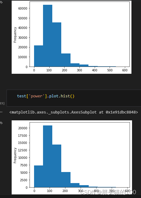

4.模型初始化和数据准备

• 这段代码展示了如何使用scikit-learn和XGBoost库进行回归建模、模型评估、参数调优和预测。
• 使用了三种不同的回归模型（随机森林、XGBoost、梯度提升树）进行性能比较。
• 对XGBoost模型进行了参数调优，以提高模型的预测性能。
• 最后，使用调优后的XGBoost模型对测试集进行预测，并将结果保存为CSV文件，以便提交。

rf = RandomForestRegressor(n_estimators=100, max_depth=8, random_state=1) 
xgb = XGBRegressor(n_stimators=150, max_depth=8, learning_rate=0.1, random_state=1)  
gbdt = GradientBoostingRegressor(subsample=0.8, random_state=1)  # subsample小于1可降低方差，但会加大偏差

X = train.drop(['price'], axis=1)
y = train['price']

#随机森林
score_rf = -1 * cross_val_score(rf,
                           X,
                           y,
                           scoring='neg_mean_absolute_error',
                           cv=5).mean()  # 取得分均值

print('随机森林模型的平均MAE为:', score_rf)

# XGBoost
score_xgb = -1 * cross_val_score(xgb,
                                X,
                                y,
                                scoring='neg_mean_absolute_error',
                                cv=5).mean()  # 取得分均值

print('XGBoost模型的平均MAE为:', score_xgb)

# 梯度提升树GBDT
score_gbdt = -1 * cross_val_score(gbdt,
                                X,
                                y,
                                scoring='neg_mean_absolute_error',
                                cv=5).mean()  # 取得分均值

print('梯度提升树模型的平均MAE为:', score_gbdt)


params = {'n_estimators': [150, 200, 250],
          'learning_rate': [0.1],
          'subsample': [0.5, 0.8]}

model = GridSearchCV(estimator=xgb,
                    param_grid=params,
                    scoring='neg_mean_absolute_error',
                    cv=3)
model.fit(X, y)

# 输出最佳参数
print('最佳参数为：\n', model.best_params_)
print('最佳分数为：\n', model.best_score_)
print('最佳模型为：\n', model.best_estimator_)

predictions = model.predict(test)
result = pd.DataFrame({'SaleID': df_test['SaleID'], 'price': predictions})
result.to_csv('My_submission.csv', index=False)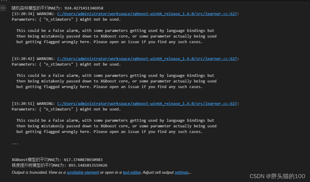

5，总结

项目准备：导入必要的模块，使用pip安装缺失的模块

1. 数据读取：
   • 使用pd.read_csv方法读取了训练集和测试集的CSV文件，指定了分隔符为空格（sep=' '）。
2. 数据预处理：
   • 删除了训练集和测试集中的SaleID列，因为它可能不是预测目标价格的必要特征。
   • 将notRepairedDamage列中的'-'替换为np.nan（表示缺失值），并将数据类型转换为float64。
   • 删除了seller和offerType列，可能因为它们对预测价格的影响不大或者包含冗余信息。
3. 探索性数据分析：
   • 使用train.info()和test.info()方法查看了训练集和测试集的基本信息，包括列名、非空值数量、数据类型等。
   • 使用train.describe()和test.describe()方法查看了数值型特征的统计描述。
4. 处理缺失值：
   • 识别了power列中大于600的异常值（可能表示数据输入错误或不合法的值），但未进行实际处理。
   • 对于model列中的缺失值，通过查找与缺失值所在行其他特征（brand, bodyType, gearbox, power）相同的行的model值，选择了出现次数最多的值进行填充（但只展示了一个示例填充）。
   • 对于bodyType列中的缺失值，选择用该列中出现次数最多的值（0.0）进行填充。
5. 数据验证：
   • 在填充model列的缺失值后，通过查看train.loc[38424, :]验证了填充结果。
   • 使用train.info()再次查看了训练集的信息，确保model和bodyType列的缺失值已被处理。
   • 分析了bodyType列中不同值的数量分布，以支持使用0.0作为缺失值的填充选择。
6. 注意事项：
   • 在处理model列的缺失值时，只展示了一个示例的填充过程，并未对所有缺失值进行自动填充。
   • 对于power列中的异常值，尚未进行实际处理，可能需要进一步分析或删除这些异常值。

后半代码总结：

1. 模型初始化：
   • 初始化了三个回归模型：随机森林（RandomForestRegressor）、XGBoost（XGBRegressor）和梯度提升树（GradientBoostingRegressor）。其中，随机森林和XGBoost模型设置了特定的参数，而梯度提升树只设置了subsample参数。
2. 数据准备：
   • 从train数据集中提取特征X（除了价格'price'以外的所有列）和目标变量y（即'price'列）。
3. 交叉验证和模型评估：
   • 使用交叉验证（cross_val_score）和平均绝对误差（MAE，通过scoring='neg_mean_absolute_error'设置）来评估三个模型的性能。每个模型都使用5折交叉验证，并输出平均MAE分数。
4. 参数调优（仅针对XGBoost）：
   • 设置了XGBoost模型的参数网格（param_grid），包括n_estimators（树的数量）、learning_rate（学习率）和subsample（子样本比例）。
   • 使用GridSearchCV进行参数调优，通过3折交叉验证搜索最佳参数组合。
   • 输出最佳参数、最佳分数和最佳模型。
5. 预测和提交：
   • 使用经过参数调优的XGBoost模型对测试集test进行预测。
   • 将预测的价格与测试集的SaleID结合，生成一个DataFrame。
   • 将这个DataFrame保存为CSV文件My_submission.csv，以便提交到可能的机器学习

    本文文章链接：python数据分析——二手车价格预测-CSDN博客