算法导论第三版第15章习题答案

最新推荐文章于 2022-12-21 09:58:19 发布

时时处处皆修行

最新推荐文章于 2022-12-21 09:58:19 发布

阅读量1.9w

点赞数 12

分类专栏： Algorithm 文章标签： python 算法导论

本文链接：https://blog.csdn.net/davidwang9527/article/details/109544199

版权

Algorithm 专栏收录该内容

8 篇文章 14 订阅

订阅专栏

2020/11/18:初稿，增加Python代码实现，修订参考文献部分错误(如15.1的第4题)

参考文献：
https://walkccc.github.io/CLRS/Chap15/
https://cs.stackexchange.com/questions/118451/why-this-greedy-algorithm-fails-in-rod-cutting-problem
https://leetcode-cn.com/problems/longest-increasing-subsequence/
https://leetcode-cn.com/problems/longest-palindromic-substring/solution/zui-chang-hui-wen-zi-chuan-by-leetcode-solution/
https://algorithms.tutorialhorizon.com/dynamic-programming-edit-distance-problem/

15 Dynamic Programming

15.1 Rod cutting

1.Show that equation (15.4) follows from equation (15.3) and the initial condition T(0)=1.

For n=0, this holds since $2^0 = 1$ .
For n>0, substituting into the recurrence, we have

$T(n) = 1 + \sum_{j=0}^{n-1}2^j = 1+(2^n -1) = 2^n$

2.Show, by means of a counterexample, that the following "greedy" strategy does not always determine an optimal way to cut rods. Define the density of a rod of length i to be $p_i / i$ , that is, its value per inch. The greedy strategy for a rod of length n cuts off a first piece of length i, where 1≤i≤n, having maximum density. It then continues by applying the greedy strategy to the remaining piece of length n−i.

Consider prices up to length 4 are $p_1=1,p_2=5,p_3=8,p_4=9$ respectively. So, densities are $d_1=1,d_2=2.5,d_3=2.67,d_4=2.25$ respectively. If we are given a rod of length 4, then an optimal way of cutting the rod to maximize revenue is 2 pieces of length 2 each, generating 5+5=10. However, greedy algorithm above will suggest cutting the rod into 2 pieces of length 3 and 1, generating revenue 8+1=9.

3.Consider a modification of the rod-cutting problem in which, in addition to a price $p_i$ for each rod, each cut incurs a fixed cost of c. The revenue associated with a solution is now the sum of the prices of the pieces minus the costs of making the cuts. Give a dynamic-programming algorithm to solve this modified problem.

We can modify BOTTOM-UP-CUT-ROD algorithm from section 15.1 as follows:

MODIFIED-CUT-ROD(p, n, c)
    let r[0..n] be a new array
    r[0] = 0
    for j = 1 to n
        q = p[j]
        for i = 1 to j - 1
            q = max(q, p[i] + r[j - i] - c)
        r[j] = q
    return r[n]

We need to account for cost c on every iteration of the loop in lines 5-6 but the last one, when i = j(no cuts).We make the loop run to j - 1 instead of j, make sure c is subtracted from the candidate revenue in line 6, then pick the greater of current best revenue q and p[j] (no cuts) in line 7.

Python Implementation:

def bottom_up_cut_pod(p,n,c):
    r = [float("-inf")] * (n + 1)
    r[0] = 0

    for j in range(1,n + 1):
        q = p[j]
        for i in range(1, j):
            q = max(q, p[i] + r[j -i] - c)
        r[j] = q

    return r[n]

p=[0,1,5,8,9,10,17,17,20,24,30]
c=1
for n in range(0,11):
    print("n={},r={}".format(n,bottom_up_cut_pod(p,n,c)))

4.Modify MEMOIZED-CUT-ROD to return not only the value but the actual solution, too.

MEMOIZED-CUT-ROD(p, n)
    let r[0..n] and s[0..n] be new arrays
    for i = 0 to n
        r[i] = -∞
    (val, s) = MEMOIZED-CUT-ROD-AUX(p, n, r, s)
    print "The optimal value is" val "and the cuts are at"
    j = n
    while j > 0
        print s[j]
        j = j - s[j]

MEMOIZED-CUT-ROD-AUX(p, n, r, s)
    if r[n] ≥ 0
        return (r[n],s)
    if n == 0
        q = 0
    else q = -∞
        for i = 1 to n
            (val, s) = MEMOIZED-CUT-ROD-AUX(p, n - i, r, s)
            if q < p[i] + val
                q = p[i] + val
                s[n] = i
    r[n] = q
    return (q, s)

Python Implementation:

def memorized_cut_pod_aux(p,n,r,s):
    if r[n] >= 0:
        return (r[n],s)
    
    if n == 0:
        q = 0
    else:
        q = float("-inf")
        for i in range(1, n+1):
            (val, s) =memorized_cut_pod_aux(p, n - i, r, s)
            if q < p[i] + val:
                q = p[i] + val
                s[n] = i
    r[n] = q

    return (q, s)

def memorized_cut_pod(p,n):
    r = [float("-inf")] * (n + 1)
    s = [float("-inf")] * (n + 1)

    val, s = memorized_cut_pod_aux(p, n, r, s)

    tmp_s = []
    i = n
    while i > 0:
        tmp_s.append(s[i])
        i = i - s[i]
    
    print('n={},r={},s={}'.format(n,val,tmp_s))

p=[0,1,5,8,9,10,17,17,20,24,30]

for n in range(0,11):
    memorized_cut_pod(p,n)

5.The Fibonacci numbers are defined by recurrence (3.22). Give an O.n/-time dynamic-programming algorithm to compute the nth Fibonacci number. Draw the subproblem graph. How many vertices and edges are in the graph?

The Fibonacci numbers are defined by recurrence (3.22). Give an O(n)-time dynamic-programming algorithm to compute the nth Fibonacci number. Draw the subproblem graph. How many vertices and edges are in the graph?

FIBONACCI(n)
    let fib[0..n] be a new array
    fib[0] = 1
    fib[1] = 1
    for i = 2 to n
        fib[i] = fib[i - 1] + fib[i - 2]
    return fib[n]

Python Implementation:

def fibonacci_dp(n):
    dp =[0]* (n + 1)
    
    dp[1] = 1

    for i in range(2,n + 1):
        dp[i] = dp[i-2] + dp[i-1]

    return dp[n]

print(fibonacci_dp(10))

There are n+1 vertices in the subproblem graph, i.e., $v_0, v_1, \dots, v_n$ .

For $v_0, v_1$ , each has 0 leaving edge.
For $v_2, v_3, \dots, v_n$ , each has 2 leaving edges.

Thus, there are 2n - 2 edges in the subproblem graph.

15.2 Matrix-chain multiplication

1.Find an optimal parenthesization of a matrix-chain product whose sequence of dimensions is 〈5,10,3,12,5,50,6〉.

((5×10)(10×3))(((3×12)(12×5))((5×50)(50×6))).

2.Give a recursive algorithm MATRIX-CHAIN-MULTIPLY(A,s,i,j) that actually performs the optimal matrix-chain multiplication, given the sequence of matrices 〈A1,A2,…,An〉, the s table computed by MATRIX-CHAIN-ORDER, and the indices i and j. (The initial call would be MATRIX-CHAIN-MULTIPLY(A,s,1,n).)

MATRIX-CHAIN-MULTIPLY(A, s, i, j)
    if i == j
        return A[i]
    if i + 1 == j
        return A[i] * A[j]
    b = MATRIX-CHAIN-MULTIPLY(A, s, i, s[i, j])
    c = MATRIX-CHAIN-MULTIPLY(A, s, s[i, j] + 1, j)
    return b * c

3.Use the substitution method to show that the solution to the recurrence (15.6) is $\Omega(2^n)$

4.Describe the subproblem graph for matrix-chain multiplication with an input chain of length nn. How many vertices does it have? How many edges does it have, and which edges are they?

5.Describe the subproblem graph for matrix-chain multiplication with an input chain of length n. How many vertices does it have? How many edges does it have, and which edges are they?

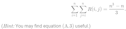
Let R(i,j) be the number of times that table entry m[i, j] is referenced while computing other table entries in a call of MATRIX-CHAIN-ORDER. Show that the total number of references for the entire table is

6.Show that a full parenthesization of an n-element expression has exactly n−1 pairs of parentheses.

We proceed by induction on the number of matrices. A single matrix has no pairs of parentheses. Assume that a full parenthesization of an n-element expression has exactly n − 1 pairs of parentheses. Given a full parenthesization of an (n+1)-element expression, there must exist some k such that we first multiply B=A1⋯Ak in some way, then multiply $C = A_{k + 1} \cdots A_{n + 1}$ in some way, then multiply B and C. By our induction hypothesis, we have k − 1 pairs of parentheses for the full parenthesization of B and n+1−k−1 pairs of parentheses for the full parenthesization of C. Adding these together, plus the pair of outer parentheses for the entire expression, yields k−1+n+1−k−1+1=(n+1)−1 parentheses, as desired.

15.3 Elements of dynamic programming

1.Which is a more efficient way to determine the optimal number of multiplications in a matrix-chain multiplication problem: enumerating all the ways of parenthesizing the product and computing the number of multiplications for each, or running RECURSIVE-MATRIX-CHAIN? Justify your answer.

Running RECURSIVE-MATRIX-CHAIN is asymptotically more efficient than enumerating all the ways of parenthesizing the product and computing the number of multiplications for each. Consider the treatment of subproblems by each approach:

For each possible place to split the matrix chain, the enumeration approach finds all ways to parenthesize the left half, finds all ways to parenthesize the right half, and looks at all possible combinations of the left half with the right half. The amount of work to look at each combination of left and right half subproblem results is thus the product of the number of ways to parenthesize the left half and the number of ways to parenthesize the right half.
For each possible place to split the matrix chain,RECURSIVE-MATRIX-CHAIN finds the best way to parenthesize the left half, finds the best way to parenthesize the right half, and combines just those two results. Thus the amount of work to combine the left and right half subproblem results is O(1).

2.Draw the recursion tree for the MERGE-SORT procedure from Section 2.3.1 on an array of 16 elements. Explain why memoization fails to speed up a good divide-and-conquer algorithm such as MERGE-SORT.

Draw a recursion tree. The MERGE-SORT procedure performs at most a single call to any pair of indices of the array that is being sorted. In other words, the subproblems do not overlap and therefore memoization will not improve the running time.

3.Consider a variant of the matrix-chain multiplication problem in which the goal is to parenthesize the sequence of matrices so as to maximize, rather than minimize, the number of scalar multiplications. Does this problem exhibit optimal substructure?

Yes, this problem also exhibits optimal substructure. If we know that we need the subproduct $(A_l \cdot A_r)$ , then we should still find the most expensive way to compute it — otherwise, we could do better by substituting in the most expensive way.

4.As stated, in dynamic programming we first solve the subproblems and then choose which of them to use in an optimal solution to the problem. Professor Capulet claims that we do not always need to solve all the subproblems in order to find an optimal solution. She suggests that we can find an optimal solution to the matrix-chain multiplication problem by always choosing the matrix $A_k$ at which to split the subproduct $A_i A_{i + 1} \cdots A_j$ (by selecting k to minimize the quantity $p_{i - 1} p_k p_j$ ) before solving the subproblems. Find an instance of the matrix-chain multiplication problem for which this greedy approach yields a suboptimal solution.

5.Suppose that in the rod-cutting problem of Section 15.1, we also had limit $l_i$ on the number of pieces of length i that we are allowed to produce, for $i = 1, 2, \ldots, n$ . Show that the optimal-substructure property described in Section 15.1 no longer holds.

The optimal substructure property doesn't hold because the number of pieces of length i used on one side of the cut affects the number allowed on the other. That is, there is information about the particular solution on one side of the cut that changes what is allowed on the other.

To make this more concrete, suppose the rod was length 4, the values were $l_1 = 2, l_2 = l_3 = l_4 = 1$ , and each piece has the same worth regardless of length. Then, if we make our first cut in the middle, we have that the optimal solution for the two rods left over is to cut it in the middle, which isn't allowed because it increases the total number of rods of length 1 to be too large.

6.Imagine that you wish to exchange one currency for another. You realize that instead of directly exchanging one currency for another, you might be better off making a series of trades through other currencies, winding up with the currency you want. Suppose that you can trade nn different currencies, numbered 1,2,…,n, where you start with currency 1 and wish to wind up with currency n. You are given, for each pair of currencies i and j , an exchange rate $r_{ij}$ , meaning that if you start with d units of currency i , you can trade for $dr_{ij}$ units of currency j. A sequence of trades may entail a commission, which depends on the number of trades you make. Let $c_k$ be the commission that you are charged when you make k trades. Show that, if $c_k = 0$ for all k=1,2,…,n, then the problem of finding the best sequence of exchanges from currency 1 to currency n exhibits optimal substructure. Then show that if commissions $c_k$ are arbitrary values, then the problem of finding the best sequence of exchanges from currency 1 to currency n does not necessarily exhibit optimal substructure.

15.4 Longest common subsequence

1.Determine an 〈1,0,0,1,0,1,0,1〉 and 〈0,1,0,1,1,0,1,1,0〉.

〈1,0,0,1,1,0〉.

2.Give pseudocode to reconstruct an LCS from the completed c table and the original sequences $X = \langle x_1, x_2, \ldots, x_m \rangle$ and $Y = \langle y_1, y_2, \ldots, y_n \rangle$ in O(m + n) time, without using the b table.

PRINT-LCS(c, X, Y, i, j)
    if c[i, j] == 0
        return
    if X[i] == Y[j]
        PRINT-LCS(c, X, Y, i - 1, j - 1)
        print X[i]
    else if c[i - 1, j] > c[i, j - 1]
        PRINT-LCS(c, X, Y, i - 1, j)
    else
        PRINT-LCS(c, X, Y, i, j - 1)

Python Implementation:

import numpy as np

def lcs_length(X,Y):
    """Calculate longest common subsequence.
    
    Longest common subsequence by dynamic programming(bottom up).
    
    Args:
        X(list): Sequence X
        Y(list): Sequence Y
    
    Returns:
        tuple: (c,b). Both c and b are matrix of (m + 1,n + 1) where m=X.length and n=Y.length.
               c[i,j] contains the length of an LCS of X[1..i] and Y[1..j],thus c[m,n] 
               contains the length of an LCS of X and Y.The procedure also maintains the 
               table b[1..m,1..n] to help us construct an optimal solution. Intuitively, 
               b[i,j]  points to the table entry corresponding to the optimal subproblem 
               solution chosen when computing c[i,j].
    """
    m = len(X)
    n = len(Y)

    b = np.zeros((m + 1, n + 1))
    c = np.zeros((m + 1, n + 1))

    for i in range(1, m + 1):
        for j in range(1, n + 1):
            if X[i-1] == Y[j-1]:
                c[i,j] = c[i - 1, j - 1] + 1
                b[i,j] = 1
            elif c[i-1, j] >= c[i, j - 1]:
                c[i,j] = c[i - 1, j]
                b[i,j] = 2
            else:
                c[i,j] = c[i, j - 1]
                b[i,j] = 3
    return (c,b)

def print_lcs(b,X,i,j):
    if i ==0 or j ==0 :
        return
    if b[i,j] == 1:
        print_lcs(b,X,i-1,j-1)
        print(X[i-1])
    elif b[i,j] == 2:
        print_lcs(b,X,i-1,j)
    else:
        print_lcs(b,X,i,j-1)

def print_lcs_with_only_c(c,X,Y,i,j):
    if c[i,j] == 0:
        return
    
    if X[i-1] == Y[j-1]:
        print_lcs_with_only_c(c,X,Y,i-1,j-1)
        print(X[i-1])
    elif c[i - 1, j] > c[i, j - 1]:
        print_lcs_with_only_c(c,X,Y,i - 1,j)
    else:
        print_lcs_with_only_c(c,X,Y,i,j - 1)
    
    return

X = ['A','B','C','B','D','A','B']
Y = ['B','D','C','A','B','A']

c, b=lcs_length(X,Y)
print('Lenghth of longest common subsequence:',c[len(X),len(Y)])
print('The longest common subsequence is :')
print_lcs(b,X,len(X),len(Y))
print('The longest common subsequence is :')
print_lcs_with_only_c(c,X,Y,len(X),len(Y))

X = [1,0,0,1,0,1,0,1]
Y = [0,1,0,1,1,0,1,1,0]
c, b=lcs_length(X,Y)
print('Lenghth of longest common subsequence:',c[len(X),len(Y)])
print('The longest common subsequence is :')
print_lcs(b,X,len(X),len(Y))
print('The longest common subsequence is :')
print_lcs_with_only_c(c,X,Y,len(X),len(Y))

Note: the result of print_lcs and print_lcs_with_only_c are different but both outputs are correct solutions.

3.Give a memoized version of LCS-LENGTH that runs in O(mn) time.

MEMOIZED-LCS-LENGTH(c,X, Y, i, j)
    if c[i, j] > -1
        return c[i, j]
    if i == 0 or j == 0
        return c[i, j] = 0
    if x[i] == y[j]
        return c[i, j] = MEMOIZED-LCS-LENGTH(X, Y, i - 1, j - 1) + 1
    return c[i, j] = max(MEMOIZED-LCS-LENGTH(X, Y, i - 1, j), MEMOIZED-LCS-LENGTH(X, Y, i, j - 1))

Python Implementation:

import numpy as np

def memorized_lcs_length(C,X,Y,i,j):
    """Calculate longest common subsequence.
    
    Longest common subsequence by dynamic programming.
    
    Args:
        C(ndarray):matrix of (m + 1,n + 1) where m=X.length and n=Y.length.
               c[i,j] contains the length of an LCS of X[1..i] and Y[1..j],thus c[m,n] 
               contains the length of an LCS of X and Y.
        X(list): Sequence X
        Y(list): Sequence Y
        i(int) : Length of X
        j(int) : Lenght of Y
    
    Returns:
        C[i,j] : the las element of matrix C, which is the length of an LCS of X and Y.
    """
    if C[i, j] > -1:
        return C[i, j]
    
    if i == 0 or j ==0 :
        return C[i,j] == 0
    
    if X[i - 1] == Y[j -1]:
        C[i, j] = memorized_lcs_length(C,X, Y, i-1, j-1) + 1
    else:
        C[i,j] = max(memorized_lcs_length(C,X,Y,i-1,j),memorized_lcs_length(C,X,Y,i,j-1))
    
    return C[i,j]

X = ['A','B','C','B','D','A','B']
Y = ['B','D','C','A','B','A']
C = (-1)*np.ones((len(X)+1,len(Y)+1))
c = memorized_lcs_length(C,X,Y,len(X),len(Y))
print('Lenghth of longest common subsequence:',c)

4.Show how to compute the length of an LCS using only $2 \cdot \min(m, n)$ entries in the c table plus O(1) additional space. Then show how to do the same thing, but using min(m,n) entries plus O(1) additional space.

Since we only use the previous row of the c table to compute the current row, we compute as normal, but when we go to compute row k, we free row k - 2 since we will never need it again to compute the length. To use even less space, observe that to compute c[i, j], all we need are the entries c[i − 1, j], c[i−1,j−1], and c[i,j−1]. Thus, we can free up entry-by-entry those from the previous row which we will never need again, reducing the space requirement to min(m,n). Computing the next entry from the three that it depends on takes O(1) time and space.

5.Give an $O(n^2)$ -time algorithm to find the longest monotonically increasing subsequence of a sequence of n numbers.

解法1：Given a list of numbers L, make a copy of L called L' and then sort L'. Then, just run the LCS algorithm on these two lists. The longest common subsequence must be monotone increasing because it is a subsequence of L' which is sorted. It is also the longest monotone increasing subsequence because being a subsequence of L' only adds the restriction that the subsequence must be monotone increasing. Since |L| = |L'| = n, and sorting L can be done in o $(n^2)$ time, the final running time will be O(|L'|) = $O(n^2)$

解法2：定义 dp[i] 为考虑前 ii 个元素，以第 i个数字结尾的最长上升子序列的长度，注意 nums[i] 必须被选取。我们从小到大计算 dp[] 数组的值，在计算 dp[i] 之前，我们已经计算出 dp[0…i−1] 的值，则状态转移方程为：

$dp[i] = \text{max}(dp[j]) + 1,$ 其中 $\, 0 \leq j < i \,$ 且 $\, \textit{num}[j]<\textit{num}[i]$

即考虑往dp[0…i−1] 中最长的上升子序列后面再加一个 nums[i]。由于 dp[j]代表nums[0…j] 中以 nums[j] 结尾的最长上升子序列，所以如果能从 dp[j] 这个状态转移过来，那么 nums[i] 必然要大于 nums[j]，才能将nums[i] 放在nums[j] 后面以形成更长的上升子序列。

最后，整个数组的最长上升子序列即所有 dp[i]中的最大值。

class Solution:
    def lengthOfLIS(self, nums):
        n = len(nums)
        
        if n < 2:
            return n
        
        dp = [1] * n

        for i in range(1, n):
            for j in range(0,i):
                if nums[j] < nums[i]:
                    dp[i] = max(dp[j]+1,dp[i])

        return max(dp)

s = Solution()
print(s.lengthOfLIS([4,10,4,3,8,9]))

6.Give an O(nlgn)-time algorithm to find the longest monotonically increasing subsequence of a sequence of n numbers.Hint: Observe that the last element of a candidate subsequence of length i is at least as large as the last element of a candidate subsequence of length i−1. Maintain candidate subsequences by linking them through the input sequence.)

tails is an array storing the smallest tail of all increasing subsequences with length i+1 in tails[i]. For example, say we have nums = [4,5,6,3], then all the available increasing subsequences are

len = 1   :      [4], [5], [6], [3]   => tails[0] = 3
len = 2   :      [4, 5], [5, 6]       => tails[1] = 5
len = 3   :      [4, 5, 6]            => tails[2] = 6

We can easily prove that tails is a increasing array. Therefore it is possible to do a binary search in tails array to find the one needs update.Each time we only do one of the two:

(1) if x is larger than all tails, append it, increase the size by 1
(2) if tails[i-1] < x <= tails[i], update tails[i]

Doing so will maintain the tails invariant. The the final answer is just the size.

class Solution:
    def lengthOfLIS(self, nums: [int]) -> int:
        tails, res = [0] * len(nums), 0
        for num in nums:
            i, j = 0, res
            while i < j:
                m = (i + j) // 2
                if tails[m] < num: 
                    i = m + 1 # 如果要求非严格递增，将此行 '<' 改为 '<=' 即可。
                else: 
                    j = m
            tails[i] = num
            if j == res: 
                res += 1
        return res

s = Solution()
print(s.lengthOfLIS([4,10,4,3,8,9]))

15.5 Optimal binary search trees

1.Write pseudocode for the procedure CONSTRUCT-OPTIMAL-BST(root) which, given the table root, outputs the structure of an optimal binary search tree. For the example in Figure 15.10, your procedure should print out the structure

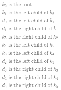
corresponding to the optimal binary search tree shown in Figure 15.9(b).

CONSTRUCT-OPTIMAL-BST(root, i, j, last)
    if i == j
        return
    if last == 0
        print root[i, j] + "is the root"
    else if j < last:
        print root[i, j] + "is the left child of" + last
    else
        print root[i, j] + "is the right child of" + last
    CONSTRUCT-OPTIMAL-BST(root, i, root[i, j] - 1, root[i, j])
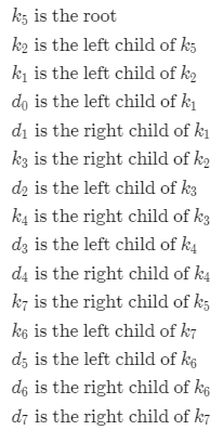
    CONSTRUCT-OPTIMAL-BST(root, root[i, j] + 1, j, root[i, j])

2.Determine the cost and structure of an optimal binary search tree for a set of n=7 keys with the following probabilities

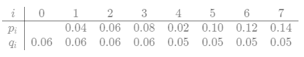
Cost is 3.12.

3.Suppose that instead of maintaining the table w[i,j], we computed the value of w(i,j) directly from equation(15.12) in line 9 of OPTIMAL-BST and used this computed value in line 11. How would this change affect the asymptotic running time of OPTIMAL-BST?

Each of the $\Theta(n^2)$ values of w[i,j] would require computing those two sums, both of which can be of sizeO(n), so, the asymptotic runtime would increase to $O(n^3)$ .

4.Knuth [212] has shown that there are always roots of optimal subtrees such that root[i,j−1]≤root[i,j]≤root[i+1,j] for all 1≤i<j≤n. Use this fact to modify the OPTIMAL-BST procedure to run in $\Theta(n^2)$ time.

Change the for loop of line 10 in OPTIMAL-BST to

    for r = r[i, j - 1] to r[i + 1, j]

Knuth's result implies that it is sufficient to only check these values because optimal root found in this range is in fact the optimal root of some binary search tree. The time spent within the for loop of line 6 is now Θ(n). This is because the bounds on rr in the new for loop of line 10 are nonoverlapping.

To see this, suppose we have fixed l and i. On one iteration of the for loop of line 6, the upper bound on r is

r[i+1,j]=r[i+1,i+l−1].

When we increment i by 1 we increase j by 1. However, the lower bound on r for the next iteration subtracts this, so the lower bound on the next iteration is

r[i + 1, j + 1 - 1] = r[i + 1, j].

Thus, the total time spent in the for loop of line 6 is Θ(n). Since we iterate the outer for loop of line 5 n times, the total runtime is $\Theta(n^2)$ .

Problems

1 Longest simple path in a directed acyclic graph.Suppose that we are given a directed acyclic graph G = (V, E) with real-valued edge weights and two distinguished vertices s and t . Describe a dynamic-programming approach for finding a longest weighted simple path from s to t. What does the subproblem graph look like? What is the efficiency of your algorithm?

Since any longest simple path must start by going through some edge out of s, and thereafter cannot pass through s because it must be simple, that is,

$\text{LONGEST}(G, s, t) = 1 + \max_{s~s'} \text\{LONGEST(G|_{V\backslash\{s\}}, s', t)\}$

with the base case that if s = t then we have a length of 0.

A naive bound would be to say that since the graph we are considering is a subset of the vertices, and the other two arguments to the substructure are distinguished vertices, then, the runtime will be $O(|V|^2 2^{|V|})$ . We can see that we will actually have to consider this many possible subproblems by taking ∣G∣ to be the complete graph on ∣V∣ vertices.

2.Longest palindrome subsequence: A palindrome is a nonempty string over some alphabet that reads the same forward and backward. Examples of palindromes are all strings of length 1, civic, racecar, andaibohphobia (fear of palindromes).Give an efficient algorithm to find the longest palindrome that is a subsequence of a given input string. For example, given the input character, your algorithm should return carac. What is the running time of your algorithm?

对于一个子串而言，如果它是回文串，并且长度大于 2，那么将它首尾的两个字母去除之后，它仍然是个回文串。例如对于字符串”ababa”，如果我们已经知道 “bab” 是回文串，那么 “ababa” 一定是回文串，这是因为它的首尾两个字母都是“a”。根据这样的思路，我们就可以用动态规划的方法解决本题。我们用 P(i,j) 表示字符串 s 的第 i 到 j 个字母组成的串（下文表示成 s[i:j]）是否为回文串：

这里的「其它情况」包含两种可能性：

s[i,j] 本身不是一个回文串；
i>j，此时 s[i, j]本身不合法。

那么我们就可以写出动态规划的状态转移方程：

也就是说，只有 s[i+1:j-1]是回文串，并且 s 的第 i 和 j 个字母相同时，s[i:j]才会是回文串。

上文的所有讨论是建立在子串长度大于 2 的前提之上的，我们还需要考虑动态规划中的边界条件，即子串的长度为 1 或 2。对于长度为 1 的子串，它显然是个回文串；对于长度为 2 的子串，只要它的两个字母相同，它就是一个回文串。因此我们就可以写出动态规划的边界条件：

根据这个思路，我们就可以完成动态规划了，最终的答案即为所有P(i,j)=true 中 j-i+1（即子串长度）的最大值。注意：在状态转移方程中，我们是从长度较短的字符串向长度较长的字符串进行转移的，因此一定要注意动态规划的循环顺序。

Python代码实现：

class Solution_dp:
    def longestPalindrome(self, s):

        n = len(s)
        dp = [[False]*n for _ in range(n)]
        ans =""

        for l in range(1, n + 1):
            for i in range(0, n - l + 1):
                j = i + l - 1

                if l == 1:
                    dp[i][j] = True
                elif l == 2:
                    dp[i][j] = (s[i] == s[j])
                else:
                    dp[i][j] = (dp[i + 1][j - 1] and s[i] == s[j])
                
                if dp[i][j] and l >= len(ans):
                    ans = s[i:j + 1]
        
        return ans

s = Solution_dp()
print(s.longestPalindrome("babad"))
print(s.longestPalindrome("cbbd"))

3.Bitonic euclidean: In the euclidean traveling-salesman problem, we are given a set of nn points in the plane, and we wish to find the shortest closed tour that connects all n points. Figure 15.11(a) shows the solution to a 77-point problem. The general problem is NP-hard, and its solution is therefore believed to require more than polynomial time (see Chapter 34).

J. L. Bentley has suggested that we simplify the problem by restricting our attention to bitonic tours, that is, tours that start at the leftmost point, go strictly rightward to the rightmost point, and then go strictly leftward back to the starting point. Figure 15.11(b) shows the shortest bitonic tour of the same 77 points. In this case, a polynomial-time algorithm is possible.

Describe an $O(n^2)$ -time algorithm for determining an optimal bitonic tour. You may assume that no two points have the same xx-coordinate and that all operations on real numbers take unit time.Hint: Scan left to right, maintaining optimal possibilities for the two parts of the tour.)

First sort all the points based on their $x$ coordinate. To index our subproblem, we will give the rightmost point for both the path going to the left and the path going to the right. Then, we have that the desired result will be the subproblem indexed by $v$ , where $v$ is the rightmost point.

Suppose by symmetry that we are further along on the left-going path, that the leftmost path is going to the ith one and the right going path is going until the jjth one. Then, if we have that i > j + 1, then we have that the cost must be the distance from the i−1st point to the ith plus the solution to the subproblem obtained where we replace i with i − 1. There can be at most $O(n^2)$ of these subproblem, but solving them only requires considering a constant number of cases. The other possibility for a subproblem is that $j \le i \le j + 1$ . In this case, we consider for every k from 1 to j the subproblem where we replace i with k plus the cost from kth point to the ith point and take the minimum over all of them. This case requires considering O(n) things, but there are only O(n) such cases. So, the final runtime is $O(n^2$ ).

4.Printing neatly. Consider the problem of neatly printing a paragraph with a monospaced font (all characters having the same width) on a printer. The input text is a sequence of n words of lengths $l_1, l_2, \ldots, l_n$ , measured in characters. We want to print this paragraph neatly on a number of lines that hold a maximum of M characters each. Our criterion of "neatness" is as follows. If a given line contains words i through j, where $i \le j$ , and we leave exactly one space between words, the number of extra space characters at the end of the line is $M - j + i - \sum_{k = i}^j l_k$ , which must be nonnegative so that the words fit on the line. We wish to minimize the sum, over all lines except the last, of the cubes of the numbers of extra space characters at the ends of lines. Give a dynamic-programming algorithm to print a paragraph of nn words neatly on a printer. Analyze the running time and space requirements of your algorithm.

First observe that the problem exhibits optimal substructure in the following way: Suppose we know that an optimal solution has kk words on the first line. Then we must solve the subproblem of printing neatly words $l_{k + 1}, \dots, l_n$ . We build a table of optimal solutions solutions to solve the problem using dynamic programming. If $n - 1 + \sum_{k = 1}^n l_k < M$ then put all words on a single line for an optimal solution. In the following algorithm PRINT-NEATLY(n), C[k] contains the cost of printing neatly words $l_k$ through $l_n$ . We can determine the cost of an optimal solution upon termination by examining C[1]. The entry P[k] contains the position of the last word which should appear on the first line of the optimal solution of words $l_1, l_2, \dots, l_n$ . Thus, to obtain the optimal way to place the words, we make $L_{P[1]}$ the last word on the first line, $l_{P[P[1]]}$ the last word on the second line, and so on.

PRINT-NEATLY(n)
    let P[1..n] and C[1..n] be new tables
    for k = n downto 1
        if sum_{i = k}^n l_i + n - k < M
            C[k] = 0
        q = ∞
        for j = 1 downto n - k
            if sum_{m = 1}^j l_{k + j} + j - 1 < M and (M - sum_{m = 1}^j l_{k + j} + j - 1) + C[k + j + 1] < q
                q = (M - sum_{m = 1}^j l_{k + j} + j - 1) + C[k + j + 1]
                P[k] = k + j
        C[k] = q

5.Edit Distance:

Each of the transformation operations has an associated cost. The cost of an operation depends on the specific application, but we assume that each operation's cost is a constant that is known to us. We also assume that the individual costs of the copy and replace operations are less than the combined costs of the delete and insert operations; otherwise, the copy and replace operations would not be used. The cost of a given sequence of transformation operations is the sum of the costs of the individual operations in the sequence. For the sequence above, the cost of transforming \text{algorithm}algorithm to \text{altruistic}altruistic is

3⋅ cost(copy)) + cost(replace) + cost(delete) + (4⋅ cost(insert)) + cost(twiddle) + cost(kill).

Since twiddles and kills have infinite costs, we will have neither of them in a minimal cost solution. The final value for the alignment will be the negative of the minimum cost sequence of edits.

EDIT(x, y, i, j)
    let m = x.length
    let n = y.length
    if i == m
        return (n - j)cost(insert)
    if j == n
        return min{(m - i)cost(delete), cost(kill)}
    initialize o1, ..., o5 to ∞
    if x[i] == y[j]
        o1 = cost(copy) + EDIT(x, y, i + 1, j + 1)
    o2 = cost(replace) + EDIT(x, y, i + 1, j + 1)
    o3 = cost(delete) + EDIT(x, y, i + 1, j)
    o4 = cost(insert) + EDIT(x, y, i, j + 1)
    if i < m - 1 and j < n - 1
        if x[i] == y[j + 1] and x[i + 1] == y[j]
            o5 = cost(twiddle) + EDIT(x, y, i + 2, j + 2)
    return min_{i ∈ [5]}{o_i}

Approach:

Start comparing one character at a time in both strings. Here we are comparing string from right to left (backwards).

Let’s say given strings are s1 and s2 with lengths m and n respectively.

case 1: last characters are same, ignore the last character.
Recursively solve for m-1, n-1
case 2: last characters are not same then try all the possible operations recursively.

a).Insert a character into s1 (same as last character in string s2 so that last character in both the strings are same): now s1 length will be m+1, s2 length : n, ignore the last character and Recursively solve for m, n-1.

b).Remove the last character from string s1. now s1 length will be m-1, s2 length : n, Recursively solve for m-1, n.

c).Replace last character into s1 (same as last character in string s2 so that last character in both the strings are same): s1 length will be m, s2 length : n, ignore the last character and Recursively solve for m-1, n-1.

choose the minimum of ( a, b, c).

Python Implementation:

def levenshtein_dp(s, t):
    m, n = len(s), len(t)
    table = [[0] * (n) for _ in range(m)]

    for i in range(n):
        if s[0] == t[i]:
            table[0][i] = i - 0
        elif i != 0:
            table[0][i] = table[0][i - 1] + 1
        else:
            table[0][i] = 1

    for i in range(m):
        if s[i] == t[0]:
            table[i][0] = i - 0
        elif i != 0:
            table[i][0] = table[i - 1][0] + 1
        else:
            table[i][0] = 1

    for i in range(1, m):
        for j in range(1, n):
            if s[i]!=t[j]:
                table[i][j] = min(1 + table[i - 1][j], 1 + table[i][j - 1], int(s[i] != t[j]) + table[i - 1][j - 1])
            else:
                table[i][j] = table[i - 1][j - 1]
    print(table)
    return table[-1][-1]

s = "mitcmu"
t = "mtacnu"
print(levenshtein_dp(s, t))

6.Planning a company party: Professor Stewart is consulting for the president of a corporation that is planning a company party. The company has a hierarchical structure; that is, the supervisor relation forms a tree rooted at the president. The personnel office has ranked each employee with a conviviality rating, which is a real number. In order to make the party fun for all attendees, the president does not want both an employee and his or her immediate supervisor to attend. Professor Stewart is given the tree that describes the structure of the corporation, using the left-child, right-sibling representation described in Section 10.4. Each node of the tree holds, in addition to the pointers, the name of an employee and that employee's conviviality ranking. Describe an algorithm to make up a guest list that maximizes the sum of the conviviality ratings of the guests. Analyze the running time of your algorithm.

The problem exhibits optimal substructure in the following way: If the root r is included in an optimal solution, then we must solve the optimal subproblems rooted at the grandchildren of r. If r is not included, then we must solve the optimal subproblems on trees rooted at the children of r. The dynamic programming algorithm to solve this problem works as follows: We make a table C indexed by vertices which tells us the optimal conviviality ranking of a guest list obtained from the subtree with root at that vertex. We also make a table G such that G[i] tells us the guest list we would use when vertex i is at the root. Let T be the tree of guests. To solve the problem, we need to examine the guest list stored at G[T.root]. First solve the problem at each leaf L. If the conviviality ranking at L is positive, G[L]={L} and C[L] = L.conviv. Otherwise G[L]=∅ and C[L]=0. Iteratively solve the subproblems located at parents of nodes at which the subproblem has been solved. In general for a node xx,

$C[x] = \min(\sum_{y\text{ is a child of } x} C[y], \sum_{y\text{ is a grandchild of } x} C[y])$

The runtime of the algorithm is $O(n^2)$ where n is the number of vertices, because we solve n subproblems, each in constant time, but the tree traversals required to find the appropriate next node to solve could take linear time.

7.Viterbi algorithm

We can use dynamic programming on a directed graph )G=(V,E) for speech recognition. Each edge (u,v)∈E is labeled with a sound σ(u,v) from a finite set Σ of sounds. The labeled graph is a formal model of a person speaking a restricted language. Each path in the graph starting from a distinguished vertex $v_0 \in V$ corresponds to a possible sequence of sounds producted by the model. We define the label of a directed path to be the concatenation of the labels of the edges on that path.

a. Our substructure will consist of trying to find suffixes of s of length one less starting at all the edges leaving v_0v0 with label \sigma_0σ0. if any of them have a solution, then, there is a solution. If none do, then there is none. See the algorithm \text{VITERBI}VITERBI for details.

VITERBI(G, s, v[0])
    if s.length = 0
        return v[0]
    for edges(v[0], v[1]) in V for some v[1]
        if sigma(v[0], v[1]) = sigma[1]
            res = VITERBI(G, (sigma[2], ..., sigma[k]), v[1])
            if res != NO-SUCH-PATH
                return (v[0], res)
    return NO-SUCH-PATH

Since the subproblems are indexed by a suffix of ss (of which there are only k) and a vertex in the graph, there are at most O(k|V|)) different possible arguments. Since each run may require testing a edge going to every other vertex, and each iteration of the for loop takes at most a constant amount of time other than the call toPROB-VITERBI, the final runtime is $O(k|V|^2)$ .

b. For this modification, we will need to try all the possible edges leaving from $v_0$ instead of stopping as soon as we find one that works. The substructure is very similar. We'll make it so that instead of just returning the sequence, we'll have the algorithm also return the probability of that maximum probability sequence, calling the fields seq and prob respectively. See the algorithm PROB-VITERBI.

Since the runtime is indexed by the same things, we have that we will call it with at most O(k∣V∣) different possible arguments. Since each run may require testing a edge going to every other vertex, and each iteration of the for loop takes at most a constant amount of time other than the call to PROB-VITERBI, the final runtime is $O(k|V|^2)$ .

PROB-VITERBI(G, s, v[0])
    if s.length = 0
        return v[0]
    sols.seq = NO-SUCH-PATH
    sols.prob = 0
    for edges(v[0], v[1]) in V for some v[1]
        if sigma(v[0], v[1]) = sigma[1]
            res = PROB-VITERBI(G, (sigma[2], ..., sigma[k]), v[1])
            if p(v[0], v[1]) * res.prob ≥ sols.prob
                sols.prob = p(v[0], v[1]) * res.prob and sols.seq = v[0], res.seq
    return sols

8.Image compression by seam carving

SEAM(A)
    let D[1..m, 1..n] be a table with zeros
    let S[1..m, 1..n] be a table with empty lists
    for i = 1 to n
        S[1, i] = (1, i)
        D[1, i] = d_{1i}
    for i = 2 to m
        for j = 1 to n
            if j == 1 // left-edge case
                if D[i - 1, j] < D[i - 1, j + 1]
                    D[i, j] = D[i - 1, j] + d_{ij}
                    S[i, j] = S[i - 1, j].insert(i, j)
                else
                    D[i, j] = D[i - 1, j + 1] + d_{ij}
                    S[i, j] = S[i - 1, j + 1].insert(i, j)
            else if j == n // right-edge case
                if D[i - 1, j - 1] < D[i - 1, j]
                    D[i, j] = D[i - 1, j - 1] + d_{ij}
                    S[i, j] = S[i - 1, j - 1].insert(i, j)
                else
                    D[i, j] = D[i - 1, j] + d_{ij}
                    S[i, j] = S[i - 1, j].insert(i, j)
            x = MIN(D[i - 1, j - 1], D[i - 1, j], D[i - 1, j + 1])
            D[i, j] = D[i - 1, j + x]
            S[i, j] = S[i - 1, j + x].insert(i, j)
    q = 1
    for j = 1 to n
        if D[m, j] < D[m, q]
            q = j
    print(S[m, q])

9.Breaking a string. A certain string-processing language allows a programmer to break a string into two pieces. Because this operation copies the string, it costs nn time units to break a string of nn characters into two pieces. Suppose a programmer wants to break a string into many pieces. The order in which the breaks occur can affect the total amount of time used. For example, suppose that the programmer wants to break a 20-character string after characters 2, 8, and 10 (numbering the characters in ascending order from the left-hand end, starting from 1). If she programs the breaks to occur in left-to-right order, then the first break costs 20 time units, the second break costs 18 time units (breaking the string from characters 3 to 20 at character 8), and the third break costs 12 time units, totaling 50 time units. If she programs the breaks to occur in right-to-left order, however, then the first break costs 20 time units, the second break costs 10 time units, and the third break costs 8 time units, totaling 38 time units. In yet another order, she could break first at 8 (costing 20), then break the left piece at 2 (costing 8), and finally the right piece at 10 (costing 12), for a total cost of 40.

Design an algorithm that, given the numbers of characters after which to break, determines a least-cost way to sequence those breaks. More formally, given a string S with n characters and an array L[1..m] containing the break points, compute the lowest cost for a sequence of breaks, along with a sequence of breaks that achieves this cost.

The subproblems will be indexed by contiguous subarrays of the arrays of cuts needed to be made. We try making each possible cut, and take the one with cheapest cost. Since there arem to try, and there are at most $m^2$ possible things to index the subproblems with, we have that the m dependence is that the solution is $O(m^3)$ . Also, since each of the additions is of a number that is O(n), each of the iterations of the for loop may take time $O(\lg n + \lg m)$ , so, the final runtime is $O(m^3 \lg n)$ . The given algorithm will return (cost, seq) where cost is the cost of the cheapest sequence, andand seq is the sequence of cuts to make.

CUT-STRING(L, i, j, l, r)
    if l == r
        return (0, [])
    minCost = ∞
    for k = i to j
        if l + r + CUT-STRING(L, i, k, l, L[k]).cost + CUT-STRING(L, k, j, L[k], j).cost < minCost
            minCost = r - l + CUT-STRING(L, i, k, l, L[k]).cost + CUT-STRING(L, k + 1, j, L[k], j).cost
            minSeq = L[k] + CUT-STRING(L, i, k, l, L[k]) + CUT-STRING(L, i, k + 1, l, L[k])
    return (minCost, minSeq)

Sample call: ``cpp L = [3, 8, 10] S = 20 CUT-STRING(L, 0, len(L), 0, s) ```

10.Planning an investment strategy.Your knowledge of algorithms helps you obtain an exciting job with the Acme Computer Company, along with a $10,000 signing bonus. You decide to invest this money with the goal of maximizing your return at the end of 10 years. You decide to use the Amalgamated Investment Company to manage your investments. Amalgamated Investments requires you to observe the following rules. It offers n different investments, numbered 1 through n. In each year j, investment i provides a return rate of $r_{ij}$ . In other words, if you invest dd dollars in investment i in year j, then at the end of year j , you have $dr_{ij}$ dollars. The return rates are guaranteed, that is, you are given all the return rates for the next 10 years for each investment. You make investment decisions only once per year. At the end of each year, you can leave the money made in the previous year in the same investments, or you can shift money to other investments, by either shifting money between existing investments or moving money to a new investement. If you do not move your money between two consecutive years, you pay a fee of $f_1$ dollars, whereas if you switch your money, you pay a fee of $f_2$ dollars, where $f_2 > f_1$ .

a. The problem, as stated, allows you to invest your money inmultiple investments in each year. Prove that there exists an optimal investment strategy that, in each year, puts all the money into a single investment. (Recall that an optimal investment strategy maximizes the amount of money after 10 years and is not concerned with any other objectives, such as minimizing risk.)

b. Prove that the problem of planning your optimal investment strategy exhibits optimal substructure.

c. Design an algorithm that plans your optimal investment strategy. What is the running time of your algorithm?

d. Suppose that Amalgamated Investments imposed the additional restriction that, at any point, you can have no more than $15,000 in any one investment. Show that the problem of maximizing your income at the end of 10 years no longer exhibits optimal substructure.

INVEST(d, n)
    let I[1..10] and R[1..10] be new tables
    for k = 10 downto 1
        q = 1
        for i = 1 to n
            if r[i, k] > r[q, k]   // i now holds the investment which looks best for a given year
                q = i
        if R[k + 1] + dr_{I[k + 1]k} - f[1] > R[k + 1] +  dr[q, k] - f[2]  // If revenue is greater when money is not moved
            R[k] = R[k + 1] + dr_{I[k + 1]k} - f[1]
            I[k] = I[k + 1]
        else
            R[k] = R[k + 1] + dr[q, k] - f[2]
            I[k] = q
    return I as an optimal stategy with return R[1]

d. The previous investment strategy was independent of the amount of money you started with. When there is a cap on the amount you can invest, the amount you have to invest in the next year becomes relevant. If we know the year-one-strategy of an optimal investment, and we know that we need to move money after the first year, we're left with the problem of investing a different initial amount of money, so we'd have to solve a subproblem for every possible initial amount of money. Since there is no bound on the returns, there's also no bound on the number of subproblems we need to solve.

11.Inventory planning

Our subproblems will be indexed by and integer i∈[n] and another integer j∈[D]. i will indicate how many months have passed, that is, we will restrict ourselves to only caring about $(d_i, \dots, d_n)$ . j will indicate how many machines we have in stock initially. Then, the recurrence we will use will try producing all possible numbers of machines from 1 to [D]. Since the index space has size O(nD) and we are only running through and taking the minimum cost from D many options when computing a particular subproblem, the total runtime will be $O(nD^2)$ .

12.Signing free-agent baseball players

Suppose that you are the general manager for a major-league baseball team. During the off-season, you need to sign some free-agent players for your team. The team owner has given you a budget of $\$X$$ to spend on free agents. You are allowed to spend less than $X altogether, but the owner will fire you if you spend any more than $\$X$ .

You are considering N different positions, and for each position, P free-agent players who play that position are available. Because you do not want to overload your roster with too many players at any position, for each position you may sign at most one free agent who plays that position. (If you do not sign any players at a particular position, then you plan to stick with the players you already have at that position.)

To determine how valuable a player is going to be, you decide to use a sabermetric statistic known as "VORP", or "value over replacement player". A player with a higher VORP is more valuable than a player with a lower VORP. A player with a higher VORP is not necessarily more expensive to sign than a player with a lower VORP, because factors other than a player's value determine how much it costs to sign him.

For each available free-agent player, you have three pieces of information:

the player's position,
the amount of money it will cost to sign the player, and
the player's \text{VORP}VORP.

Devise an algorithm that maximizes the total VORP of the players you sign while spending no more than $X altogether. You may assume that each player signs for a multiple of 100,000. Your algorithm should output the total VORP of the players you sign, the total amount of money you spend, and a list of which players you sign. Analyze the running time and space requirement of your algorithm.

We will make an N+1 by X + 1 by P + 1 table. The runtime of the algorithm is O(NXP).

BASEBALL(N, X, P)
    initialize a table B of size (N + 1) by (X + 1)
    initialize an array P of length N
    for i = 0 to N
        B[i, 0] = 0
    for j = 1 to X
        B[0, j] = 0
    for i = 1 to N
        for j = 1 to X
            if j < i.cost
                B[i, j] = B[i - 1, j]
            q = B[i - 1, j]
            p = 0
            for k = 1 to P
                if j >= i.cost
                    t = B[i - 1, j - i.cost] + i.value
                    if t > q
                        q = t
                        p = k
            B[i, j] = q
            P[i] = p
    print("The total VORP is", B[N, X], "and the players are:")
    i = N
    j = X
    C = 0
    for k = 1 to N // prints the players from the table
        if B[i, j] != B[i - 1, j]
            print(P[i])
            j = j - i.cost
            C = C + i.cost
        i = i - 1
    print("The total cost is", C)