deeplearning.ai 吴恩达网上课程学习（八）——深层神经网络分类代码实战

本文将学习如何利用Python的来实现多个隐藏层的图片分类问题：用两层和多层神经网络实现是否是猫图片的分类。

本文的实践平台是Linux，Python3.4，基础库anaconda和spyder，

参考文章的实现平台是jupyter notebook：多层神经网络代码实战

理论知识学习请参看上篇：deeplearning.ai 吴恩达网上课程学习（七）——深层神经网络理论学习

1. 流程概括：

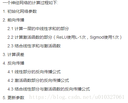
2.引入相关依赖包：

import numpy as np
import time
import h5py
import matplotlib.pyplot as plt
import scipy
from PIL import Image
from testCases_v2 import *  #提供了一些测试函数所有的数据和方法
from dnn_utils_v2 import sigmoid, sigmoid_backward, relu, relu_backward  #封装好的方法
from dnn_app_utils_v2 import *
 
plt.rcParams['figure.figsize'] = (5.0, 4.0) # set default size of plots
plt.rcParams['image.interpolation'] = 'nearest'
plt.rcParams['image.cmap'] = 'gray'
 
np.random.seed(1)

其中，sigmoid函数如下：（对输入矩阵z进行sigmoid操作，输出操作结果A和输入矩阵cache = z）

def sigmoid(Z):
    """
    Implements the sigmoid activation in numpy
    
    Arguments:
    Z -- numpy array of any shape
    
    Returns:
    A -- output of sigmoid(z), same shape as Z
    cache -- returns Z as well, useful during backpropagation
    """
    
    A = 1/(1+np.exp(-Z))
    cache = Z
    
    return A, cache

sigmoid_backward函数如下：（对单个sigmoid节点反向传播：输入dA代价函数L对a的求导，a表示的是对z的sigmoid结果，z=wx+b，cache是存储的z；输出结果是代价函数L对z的求导）

def sigmoid_backward(dA, cache):
    """
    Implement the backward propagation for a single SIGMOID unit.
 
    Arguments:
    dA -- post-activation gradient, of any shape  dL/da
    cache -- 'Z' where we store for computing backward propagation efficiently
 
    Returns:
    dZ -- Gradient of the cost with respect to Z
    """
    
    Z = cache
    
    s = 1/(1+np.exp(-Z))
    dZ = dA * s * (1-s)    #dL/dz = (dL/da)*(da/ dz) = dA*s'(z)
    
    assert (dZ.shape == Z.shape)
    
    return dZ

relu函数如下：（对输入矩阵z进行relu操作，输出操作结果A和输入矩阵cache = z ）

def relu(Z):
    """
    Implement the RELU function.
 
    Arguments:
    Z -- Output of the linear layer, of any shape
 
    Returns:
    A -- Post-activation parameter, of the same shape as Z
    cache -- a python dictionary containing "A" ; stored for computing the backward pass efficiently
    """
    
    A = np.maximum(0,Z)
    
    assert(A.shape == Z.shape)
    
    cache = Z 
    return A, cache

relu_backward函数如下：(同sigmoid_backward函数)

def relu_backward(dA, cache):
    """
    Implement the backward propagation for a single RELU unit.
 
    Arguments:
    dA -- post-activation gradient, of any shape
    cache -- 'Z' where we store for computing backward propagation efficiently
 
    Returns:
    dZ -- Gradient of the cost with respect to Z
    """
    
    Z = cache
    dZ = np.array(dA, copy=True) # just converting dz to a correct object.
    
    # When z <= 0, you should set dz to 0 as well. 
    dZ[Z <= 0] = 0
    
    assert (dZ.shape == Z.shape)
    
    return dZ

3.初始化：

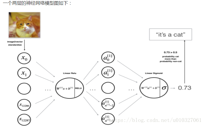
① 对于一个两层的神经网络结构

模型结构是线性->ReLU->线性->sigmod函数，初始化wi和bi的大小的矩阵

def initialize_parameters(n_x, n_h, n_y):
    """
    Argument:
    n_x -- size of the input layer
    n_h -- size of the hidden layer
    n_y -- size of the output layer
    
    Returns:
    parameters -- python dictionary containing your parameters:
                    W1 -- weight matrix of shape (n_h, n_x)
                    b1 -- bias vector of shape (n_h, 1)
                    W2 -- weight matrix of shape (n_y, n_h)
                    b2 -- bias vector of shape (n_y, 1)
    """
    
    np.random.seed(1)
    
    ### START CODE HERE ### (≈ 4 lines of code)
    W1 = np.random.randn(n_h, n_x)*0.01
    b1 = np.zeros((n_h, 1))
    W2 = np.random.randn(n_y, n_h)*0.01
    b2 = np.zeros((n_y, 1))
    ### END CODE HERE ###
    
    assert(W1.shape == (n_h, n_x))
    assert(b1.shape == (n_h, 1))
    assert(W2.shape == (n_y, n_h))
    assert(b2.shape == (n_y, 1))
    
    parameters = {"W1": W1,
                  "b1": b1,
                  "W2": W2,
                  "b2": b2}
    
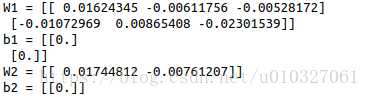
    return parameters  

验证一下：

parameters = initialize_parameters(3,2,1)
print("W1 = " + str(parameters["W1"]))
print("b1 = " + str(parameters["b1"]))
print("W2 = " + str(parameters["W2"]))
print("b2 = " + str(parameters["b2"]))

结果：

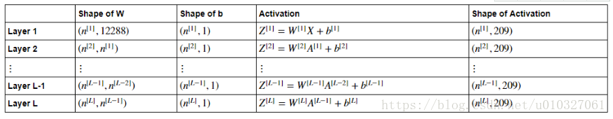
② 一个L层的神经网络的初始化：

假设X的维度为（12288,209）,表示有209个样本，每个样本有12288个特征。n[i]表示第i层神经元数量。

初始化如下：（输入的是包含神经网络每个层神经元个数的一维矩阵）

def initialize_parameters_deep(layer_dims):
    """
    Arguments:
    layer_dims -- python array (list) containing the dimensions of each layer in our network
    
    Returns:
    parameters -- python dictionary containing your parameters "W1", "b1", ..., "WL", "bL":
                    Wl -- weight matrix of shape (layer_dims[l], layer_dims[l-1])
                    bl -- bias vector of shape (layer_dims[l], 1)
    """
    
    np.random.seed(3)
    parameters = {}
    L = len(layer_dims)            # number of layers in the network
 
    for l in range(1, L):
        ### START CODE HERE ### (≈ 2 lines of code)
        parameters['W' + str(l)] = np.random.randn(layer_dims[l], layer_dims[l - 1]) / np.sqrt(layer_dims[l - 1])
        parameters['b' + str(l)] = np.zeros((layer_dims[l], 1))
        ### END CODE HERE ###
        assert(parameters['W' + str(l)].shape == (layer_dims[l], layer_dims[l-1]))
        assert(parameters['b' + str(l)].shape == (layer_dims[l], 1))
    return parameters

结果：

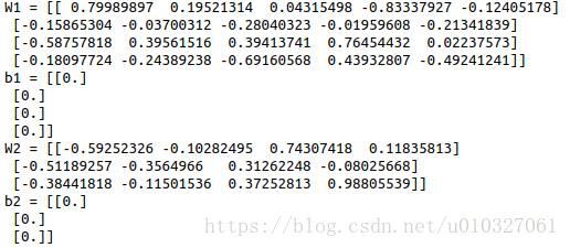
为什么关于随机数大家的结果都一样呢？那就是np.random.seed(n)的作用了，方便对随机数的预测，详细的可以参考我的前一篇文章：deeplearning.ai 吴恩达网上课程学习（六）——浅层神经网络分类代码实战Linux,TensorFlow,Python3.4,anaconda和spyder

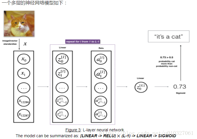
4.前向传播函数：

多层模型的前向传播计算模型如下：

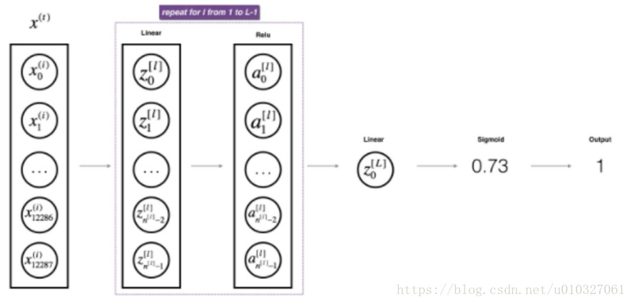
①前向传播中，线性部分计算如下：

def linear_forward(A, W, b):
    """
    Implement the linear part of a layer's forward propagation.
 
    Arguments:
    A -- activations from previous layer (or input data): (size of previous layer, number of examples)
    W -- weights matrix: numpy array of shape (size of current layer, size of previous layer)
    b -- bias vector, numpy array of shape (size of the current layer, 1)
 
    Returns:
    Z -- the input of the activation function, also called pre-activation parameter 
    cache -- a python dictionary containing "A", "W" and "b" ; stored for computing the backward pass efficiently
    """
    ### START CODE HERE ### (≈ 1 line of code)
    Z = np.dot(W, A) + b
    ### END CODE HERE ###
    assert(Z.shape == (W.shape[0], A.shape[1]))
    cache = (A, W, b)
    
    return Z, cache

测试一下：

A, W, b = linear_forward_test_case()
 
Z, linear_cache = linear_forward(A, W, b)
print("Z = " + str(Z))

其中：

def linear_forward_test_case():
    np.random.seed(1)
    A = np.random.randn(3,2)
    W = np.random.randn(1,3)
    b = np.random.randn(1,1)
    return A, W, b

结果：

Z = [[ 3.26295337 -1.23429987]]

② 线性激活函数如下：

def linear_activation_forward(A_prev, W, b, activation):
    """
    Implement the forward propagation for the LINEAR->ACTIVATION layer
 
    Arguments:
    A_prev -- activations from previous layer (or input data): (size of previous layer, number of examples)
    W -- weights matrix: numpy array of shape (size of current layer, size of previous layer)
    b -- bias vector, numpy array of shape (size of the current layer, 1)
    activation -- the activation to be used in this layer, stored as a text string: "sigmoid" or "relu"
 
    Returns:
    A -- the output of the activation function, also called the post-activation value 
    cache -- a python dictionary containing "linear_cache" and "activation_cache";
             stored for computing the backward pass efficiently
    """
    
    if activation == "sigmoid":
        # Inputs: "A_prev, W, b". Outputs: "A, activation_cache".
        ### START CODE HERE ### (≈ 2 lines of code)
        Z, linear_cache = linear_forward(A_prev, W, b)
        A, activation_cache = sigmoid(Z)
        ### END CODE HERE ###
    
    elif activation == "relu":
        # Inputs: "A_prev, W, b". Outputs: "A, activation_cache".
        ### START CODE HERE ### (≈ 2 lines of code)
        Z, linear_cache = linear_forward(A_prev, W, b)
        A, activation_cache = relu(Z)
        ### END CODE HERE ###
    
    assert (A.shape == (W.shape[0], A_prev.shape[1]))
    cache = (linear_cache, activation_cache)
 
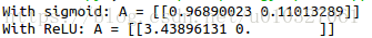
    return A, cache

测试一下：

A_prev, W, b = linear_activation_forward_test_case()
 
A, linear_activation_cache = linear_activation_forward(A_prev, W, b, activation = "sigmoid")
print("With sigmoid: A = " + str(A))
 
A, linear_activation_cache = linear_activation_forward(A_prev, W, b, activation = "relu")
print("With ReLU: A = " + str(A))

其中，linear_activation_forward_test_case函数如下：

def linear_activation_forward_test_case():
    np.random.seed(2)
    A_prev = np.random.randn(3,2)
    W = np.random.randn(1,3)
    b = np.random.randn(1,1)
    return A_prev, W, b

结果：

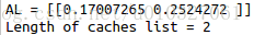
③ 前向传播函数如下：

def L_model_forward(X, parameters):
    """
    Implement forward propagation for the [LINEAR->RELU]*(L-1)->LINEAR->SIGMOID computation
    
    Arguments:
    X -- data, numpy array of shape (input size, number of examples)
    parameters -- output of initialize_parameters_deep()
    
    Returns:
    AL -- last post-activation value
    caches -- list of caches containing:
                every cache of linear_relu_forward() (there are L-1 of them, indexed from 0 to L-2)
                the cache of linear_sigmoid_forward() (there is one, indexed L-1)
    """
 
    caches = []
    A = X
    L = len(parameters) // 2                  # number of layers in the neural network
    
    # Implement [LINEAR -> RELU]*(L-1). Add "cache" to the "caches" list.
    for l in range(1, L):
        A_prev = A 
        A, cache = linear_activation_forward(A_prev, parameters['W' + str(l)], parameters['b' + str(l)], "relu")
        caches.append(cache)
    
    # Implement LINEAR -> SIGMOID. Add "cache" to the "caches" list.
    AL, cache = linear_activation_forward(A, parameters['W' + str(L)], parameters['b' + str(L)], "sigmoid")
    caches.append(cache)
    assert(AL.shape == (1,X.shape[1]))
    return AL, caches

测试一下：

X, parameters = L_model_forward_test_case()
AL, caches = L_model_forward(X, parameters)
 
print("AL = " + str(AL))
print("Length of caches list = " + str(len(caches)))

其中，L_model_forward_test_case函数如下：

def L_model_forward_test_case():
    np.random.seed(1)
    X = np.random.randn(4,2)
    W1 = np.random.randn(3,4)
    b1 = np.random.randn(3,1)
    W2 = np.random.randn(1,3)
    b2 = np.random.randn(1,1)
    parameters = {"W1": W1,
                  "b1": b1,
                  "W2": W2,
                  "b2": b2}
    
    return X, parameters

结果：

5. 计算代价函数：

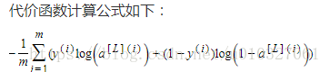
def compute_cost(AL, Y):
    """
    Implement the cost function defined by equation (7).
 
    Arguments:
    AL -- probability vector corresponding to your label predictions, shape (1, number of examples)
    Y -- true "label" vector (for example: containing 0 if non-cat, 1 if cat), shape (1, number of examples)
 
    Returns:
    cost -- cross-entropy cost
    """
    
    m = Y.shape[1]
 
    # Compute loss from aL and y.
    ### START CODE HERE ### (≈ 1 lines of code)
    cost = -np.sum(np.multiply(np.log(AL),Y) + np.multiply(np.log(1 - AL), 1 - Y)) / m
    ### END CODE HERE ###
    
    cost = np.squeeze(cost)      # To make sure your cost's shape is what we expect (e.g. this turns [[17]] into 17).
    assert(cost.shape == ())
    
    return cost

测试一下：

Y, AL = compute_cost_test_case()
 
print("cost = " + str(compute_cost(AL, Y)))

其中，compute_cost_test_case函数如下：

def compute_cost_test_case(): 
    Y = np.asarray([[1, 1, 1]]) 
    aL = np.array([[.8,.9,0.4]]) 
    return Y, aL​

结果：

6.反向传播

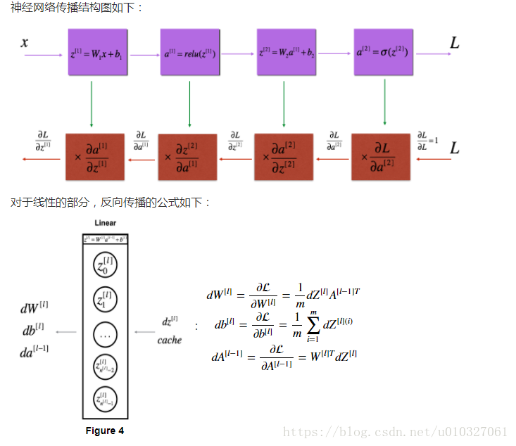
实现函数如下：

def linear_backward(dZ, cache):
    """
    Implement the linear portion of backward propagation for a single layer (layer l)
 
    Arguments:
    dZ -- Gradient of the cost with respect to the linear output (of current layer l)
    cache -- tuple of values (A_prev, W, b) coming from the forward propagation in the current layer
 
    Returns:
    dA_prev -- Gradient of the cost with respect to the activation (of the previous layer l-1), same shape as A_prev
    dW -- Gradient of the cost with respect to W (current layer l), same shape as W
    db -- Gradient of the cost with respect to b (current layer l), same shape as b
    """
    A_prev, W, b = cache
    m = A_prev.shape[1]
 
    ### START CODE HERE ### (≈ 3 lines of code)
    dW = np.dot(dZ, A_prev.T) / m
    db = np.sum(dZ, axis=1, keepdims=True) / m
    dA_prev = np.dot(W.T, dZ)
    ### END CODE HERE ###
    
    assert (dA_prev.shape == A_prev.shape)
    assert (dW.shape == W.shape)
    assert (db.shape == b.shape)
    
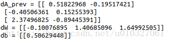
    return dA_prev, dW, db

测试一下：

dZ, linear_cache = linear_backward_test_case()
 
dA_prev, dW, db = linear_backward(dZ, linear_cache)
print ("dA_prev = "+ str(dA_prev))
print ("dW = " + str(dW))
print ("db = " + str(db))

其中，linear_backward_test_case函数如下：

def linear_backward_test_case():
    np.random.seed(1)
    dZ = np.random.randn(1,2)
    A = np.random.randn(3,2)
    W = np.random.randn(1,3)
    b = np.random.randn(1,1)
    linear_cache = (A, W, b)
    return dZ, linear_cache

结果：

接下来，我们需要计算激活函数的反向传播函数：

def linear_activation_backward(dA, cache, activation):
    """
    Implement the backward propagation for the LINEAR->ACTIVATION layer.
    
    Arguments:
    dA -- post-activation gradient for current layer l 
    cache -- tuple of values (linear_cache, activation_cache) we store for computing backward propagation efficiently
    activation -- the activation to be used in this layer, stored as a text string: "sigmoid" or "relu"
    
    Returns:
    dA_prev -- Gradient of the cost with respect to the activation (of the previous layer l-1), same shape as A_prev
    dW -- Gradient of the cost with respect to W (current layer l), same shape as W
    db -- Gradient of the cost with respect to b (current layer l), same shape as b
    """
    linear_cache, activation_cache = cache
    
    if activation == "relu":
        ### START CODE HERE ### (≈ 2 lines of code)
        dZ = relu_backward(dA, activation_cache)
        dA_prev, dW, db = linear_backward(dZ, linear_cache)
        ### END CODE HERE ###
        
    elif activation == "sigmoid":
        ### START CODE HERE ### (≈ 2 lines of code)
        dZ = sigmoid_backward(dA, activation_cache)
        dA_prev, dW, db = linear_backward(dZ, linear_cache)
        ### END CODE HERE ###
    
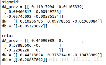
    return dA_prev, dW, db

验证一下：

AL, linear_activation_cache = linear_activation_backward_test_case()
 
dA_prev, dW, db = linear_activation_backward(AL, linear_activation_cache, activation = "sigmoid")
print ("sigmoid:")
print ("dA_prev = "+ str(dA_prev))
print ("dW = " + str(dW))
print ("db = " + str(db) + "\n")
 
dA_prev, dW, db = linear_activation_backward(AL, linear_activation_cache, activation = "relu")
print ("relu:")
print ("dA_prev = "+ str(dA_prev))
print ("dW = " + str(dW))
print ("db = " + str(db))

其中，linear_activation_backward_test_case函数如下：

def linear_activation_backward_test_case():
    np.random.seed(2)
    dA = np.random.randn(1,2)
    A = np.random.randn(3,2)
    W = np.random.randn(1,3)
    b = np.random.randn(1,1)
    Z = np.random.randn(1,2)
    linear_cache = (A, W, b)
    activation_cache = Z
    linear_activation_cache = (linear_cache, activation_cache)
    
    return dA, linear_activation_cache

结果：

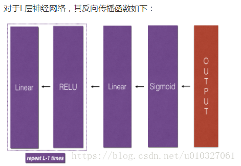
def L_model_backward(AL, Y, caches):
    """
    Implement the backward propagation for the [LINEAR->RELU] * (L-1) -> LINEAR -> SIGMOID group
    
    Arguments:
    AL -- probability vector, output of the forward propagation (L_model_forward())
    Y -- true "label" vector (containing 0 if non-cat, 1 if cat)
    caches -- list of caches containing:
                every cache of linear_activation_forward() with "relu" (it's caches[l], for l in range(L-1) i.e l = 0...L-2)
                the cache of linear_activation_forward() with "sigmoid" (it's caches[L-1])
    
    Returns:
    grads -- A dictionary with the gradients
             grads["dA" + str(l)] = ... 
             grads["dW" + str(l)] = ...
             grads["db" + str(l)] = ... 
    """
    grads = {}
    L = len(caches) # the number of layers
    m = AL.shape[1]
    Y = Y.reshape(AL.shape) # after this line, Y is the same shape as AL
    
    # Initializing the backpropagation
    ### START CODE HERE ### (1 line of code)
    dAL = - (np.divide(Y, AL) - np.divide(1 - Y, 1 - AL))
    ### END CODE HERE ###
    
    # Lth layer (SIGMOID -> LINEAR) gradients. Inputs: "AL, Y, caches". Outputs: "grads["dAL"], grads["dWL"], grads["dbL"]
    ### START CODE HERE ### (approx. 2 lines)
    current_cache = caches[L-1]
    grads["dA" + str(L)], grads["dW" + str(L)], grads["db" + str(L)] = linear_activation_backward(dAL, current_cache, "sigmoid")
    ### END CODE HERE ###
    
    for l in reversed(range(L-1)):
        # lth layer: (RELU -> LINEAR) gradients.
        # Inputs: "grads["dA" + str(l + 2)], caches". Outputs: "grads["dA" + str(l + 1)] , grads["dW" + str(l + 1)] , grads["db" + str(l + 1)] 
        ### START CODE HERE ### (approx. 5 lines)
        current_cache = caches[l]
        dA_prev_temp, dW_temp, db_temp = linear_activation_backward(grads["dA" + str(l + 2)], current_cache, "relu")
        grads["dA" + str(l + 1)] = dA_prev_temp
        grads["dW" + str(l + 1)] = dW_temp
        grads["db" + str(l + 1)] = db_temp
        ### END CODE HERE ###
 
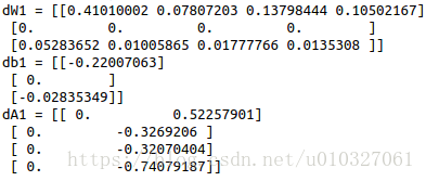
    return grads

测试一下：

AL, Y_assess, caches = L_model_backward_test_case()
grads = L_model_backward(AL, Y_assess, caches)
print ("dW1 = "+ str(grads["dW1"]))
print ("db1 = "+ str(grads["db1"]))
print ("dA1 = "+ str(grads["dA1"]))

其中，L_model_backward_test_case函数如下：

def L_model_backward_test_case():
    np.random.seed(3)
    AL = np.random.randn(1, 2)
    Y = np.array([[1, 0]])
 
    A1 = np.random.randn(4,2)
    W1 = np.random.randn(3,4)
    b1 = np.random.randn(3,1)
    Z1 = np.random.randn(3,2)
    linear_cache_activation_1 = ((A1, W1, b1), Z1)
 
    A2 = np.random.randn(3,2)
    W2 = np.random.randn(1,3)
    b2 = np.random.randn(1,1)
    Z2 = np.random.randn(1,2)
    linear_cache_activation_2 = ( (A2, W2, b2), Z2)
 
    caches = (linear_cache_activation_1, linear_cache_activation_2)
 
    return AL, Y, caches

结果：

7.更新参数：

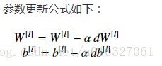
实现过程如下：

def update_parameters(parameters, grads, learning_rate):
    """
    Update parameters using gradient descent
    
    Arguments:
    parameters -- python dictionary containing your parameters 
    grads -- python dictionary containing your gradients, output of L_model_backward
    
    Returns:
    parameters -- python dictionary containing your updated parameters 
                  parameters["W" + str(l)] = ... 
                  parameters["b" + str(l)] = ...
    """
    
    L = len(parameters) // 2 # number of layers in the neural network
 
    # Update rule for each parameter. Use a for loop.
    ### START CODE HERE ### (≈ 3 lines of code)
    for l in range(L):
        parameters["W" + str(l+1)] = parameters["W" + str(l+1)] - learning_rate * grads["dW" + str(l+1)]
        parameters["b" + str(l+1)] = parameters["b" + str(l+1)] - learning_rate * grads["db" + str(l+1)]
    ### END CODE HERE ###
        
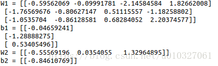
    return parameters

验证一下：

parameters, grads = update_parameters_test_case()
parameters = update_parameters(parameters, grads, 0.1)
 
print ("W1 = "+ str(parameters["W1"]))
print ("b1 = "+ str(parameters["b1"]))
print ("W2 = "+ str(parameters["W2"]))
print ("b2 = "+ str(parameters["b2"]))

其中，update_parameters_test_case函数如下：

def update_parameters_test_case():
    np.random.seed(2)
    W1 = np.random.randn(3,4)
    b1 = np.random.randn(3,1)
    W2 = np.random.randn(1,3)
    b2 = np.random.randn(1,1)
    parameters = {"W1": W1,
                  "b1": b1,
                  "W2": W2,
                  "b2": b2}
    np.random.seed(3)
    dW1 = np.random.randn(3,4)
    db1 = np.random.randn(3,1)
    dW2 = np.random.randn(1,3)
    db2 = np.random.randn(1,1)
    grads = {"dW1": dW1,
             "db1": db1,
             "dW2": dW2,
             "db2": db2}
    
    return parameters, grads

结果：

至此为止，我们已经实现该神经网络中，所有需要的函数。
接下来，我们将这些方法组合在一起，构成一个神经网络类，可以方便的使用。

8.两层神经网络模型：

定义常量：

n_x = 12288     # num_px * num_px * 3
n_h = 7
n_y = 1
layers_dims = (n_x, n_h, n_y)

两层网络模型：

def two_layer_model(X, Y, layers_dims, learning_rate = 0.0075, num_iterations = 3000, print_cost=False):
    """
    Implements a two-layer neural network: LINEAR->RELU->LINEAR->SIGMOID.
    
    Arguments:
    X -- input data, of shape (n_x, number of examples)
    Y -- true "label" vector (containing 0 if cat, 1 if non-cat), of shape (1, number of examples)
    layers_dims -- dimensions of the layers (n_x, n_h, n_y)
    num_iterations -- number of iterations of the optimization loop
    learning_rate -- learning rate of the gradient descent update rule
    print_cost -- If set to True, this will print the cost every 100 iterations 
    
    Returns:
    parameters -- a dictionary containing W1, W2, b1, and b2
    """
    
    np.random.seed(1)
    grads = {}
    costs = []                              # to keep track of the cost
    m = X.shape[1]                           # number of examples
    (n_x, n_h, n_y) = layers_dims
    
    # Initialize parameters dictionary, by calling one of the functions you'd previously implemented
    ### START CODE HERE ### (≈ 1 line of code)
    parameters = initialize_parameters(n_x, n_h, n_y)
    ### END CODE HERE ###
    
    # Get W1, b1, W2 and b2 from the dictionary parameters.
    W1 = parameters["W1"]
    b1 = parameters["b1"]
    W2 = parameters["W2"]
    b2 = parameters["b2"]
    
    # Loop (gradient descent)
 
    for i in range(0, num_iterations):
 
        # Forward propagation: LINEAR -> RELU -> LINEAR -> SIGMOID. Inputs: "X, W1, b1". Output: "A1, cache1, A2, cache2".
        ### START CODE HERE ### (≈ 2 lines of code)
        A1, cache1 = linear_activation_forward(X, W1, b1, "relu")
        A2, cache2 = linear_activation_forward(A1, W2, b2, "sigmoid")
        ### END CODE HERE ###
        
        # Compute cost
        ### START CODE HERE ### (≈ 1 line of code)
        cost = compute_cost(A2, Y)
        ### END CODE HERE ###
        
        # Initializing backward propagation
        dA2 = - (np.divide(Y, A2) - np.divide(1 - Y, 1 - A2))
        
        # Backward propagation. Inputs: "dA2, cache2, cache1". Outputs: "dA1, dW2, db2; also dA0 (not used), dW1, db1".
        ### START CODE HERE ### (≈ 2 lines of code)
        dA1, dW2, db2 = linear_activation_backward(dA2, cache2, "sigmoid")
        dA0, dW1, db1 = linear_activation_backward(dA1, cache1, "relu")
        ### END CODE HERE ###
        
        # Set grads['dWl'] to dW1, grads['db1'] to db1, grads['dW2'] to dW2, grads['db2'] to db2
        grads['dW1'] = dW1
        grads['db1'] = db1
        grads['dW2'] = dW2
        grads['db2'] = db2
        
        # Update parameters.
        ### START CODE HERE ### (approx. 1 line of code)
        parameters = update_parameters(parameters, grads, learning_rate)
        ### END CODE HERE ###
 
        # Retrieve W1, b1, W2, b2 from parameters
        W1 = parameters["W1"]
        b1 = parameters["b1"]
        W2 = parameters["W2"]
        b2 = parameters["b2"]
        
        # Print the cost every 100 training example
        if print_cost and i % 100 == 0:
            print("Cost after iteration {}: {}".format(i, np.squeeze(cost)))
        if print_cost and i % 100 == 0:
            costs.append(cost)
       
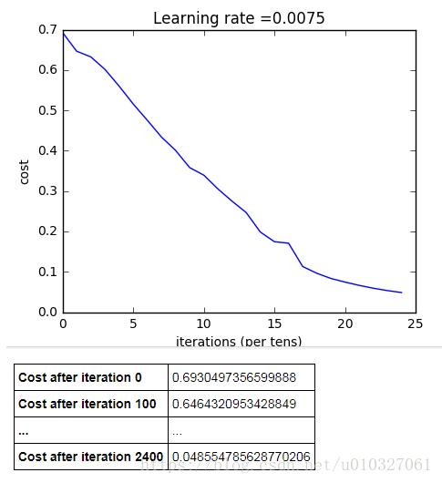
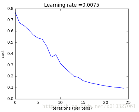
    # plot the cost
 
    plt.plot(np.squeeze(costs))
    plt.ylabel('cost')
    plt.xlabel('iterations (per tens)')
    plt.title("Learning rate =" + str(learning_rate))
    plt.show()
    
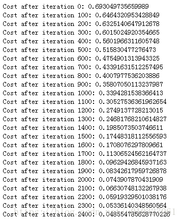
    return parameters

训练：

parameters = two_layer_model(train_x, train_y, layers_dims = (n_x, n_h, n_y), num_iterations = 2500, print_cost=True)

训练结果：

预测准确度：预测函数的实现如下：

def predict(X, y, parameters):
    """
    This function is used to predict the results of a  L-layer neural network.
    
    Arguments:
    X -- data set of examples you would like to label
    parameters -- parameters of the trained model
    
    Returns:
    p -- predictions for the given dataset X
    """
    
    m = X.shape[1]
    n = len(parameters) // 2 # number of layers in the neural network
    p = np.zeros((1,m))
    
    # Forward propagation
    probas, caches = L_model_forward(X, parameters)
 
    
    # convert probas to 0/1 predictions
    for i in range(0, probas.shape[1]):
        if probas[0,i] > 0.5:
            p[0,i] = 1
        else:
            p[0,i] = 0
    
    print("Accuracy: "  + str(float(np.sum((p == y))/m)))
        
    return p

对于训练集：

predictions_train = predict(train_x, train_y, parameters)

结果：

Accuracy:1.0

对于测试集：

predictions_test = predict(test_x, test_y, parameters)

结果：

Accuracy:0.72

9.多层神经网络：

常量初始化：

layers_dims = [12288, 20, 7, 5, 1] #  5-layer model

L层神经网络模型：

def L_layer_model(X, Y, layers_dims, learning_rate = 0.0075, num_iterations = 3000, print_cost=False):#lr was 0.009
    """
    Implements a L-layer neural network: [LINEAR->RELU]*(L-1)->LINEAR->SIGMOID.
    
    Arguments:
    X -- data, numpy array of shape (number of examples, num_px * num_px * 3)
    Y -- true "label" vector (containing 0 if cat, 1 if non-cat), of shape (1, number of examples)
    layers_dims -- list containing the input size and each layer size, of length (number of layers + 1).
    learning_rate -- learning rate of the gradient descent update rule
    num_iterations -- number of iterations of the optimization loop
    print_cost -- if True, it prints the cost every 100 steps
    
    Returns:
    parameters -- parameters learnt by the model. They can then be used to predict.
    """
 
    np.random.seed(1)
    costs = []                         # keep track of cost
    
    # Parameters initialization.
    ### START CODE HERE ###
    parameters = initialize_parameters_deep(layers_dims)
    ### END CODE HERE ###
    
    # Loop (gradient descent)
    for i in range(0, num_iterations):
 
        # Forward propagation: [LINEAR -> RELU]*(L-1) -> LINEAR -> SIGMOID.
        ### START CODE HERE ### (≈ 1 line of code)
        AL, caches = L_model_forward(X, parameters)
        ### END CODE HERE ###
        
        # Compute cost.
        ### START CODE HERE ### (≈ 1 line of code)
        cost = compute_cost(AL, Y)
        ### END CODE HERE ###
    
        # Backward propagation.
        ### START CODE HERE ### (≈ 1 line of code)
        grads = L_model_backward(AL, Y, caches)
        ### END CODE HERE ###
 
        # Update parameters.
        ### START CODE HERE ### (≈ 1 line of code)
        parameters = update_parameters(parameters, grads, learning_rate)
        ### END CODE HERE ###
                
        # Print the cost every 100 training example
        if print_cost and i % 100 == 0:
            print ("Cost after iteration %i: %f" %(i, cost))
        if print_cost and i % 100 == 0:
            costs.append(cost)
            
    # plot the cost
    plt.plot(np.squeeze(costs))
    plt.ylabel('cost')
    plt.xlabel('iterations (per tens)')
    plt.title("Learning rate =" + str(learning_rate))
    plt.show()
    
    return parameters

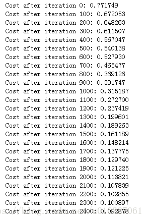
训练：

parameters = L_layer_model(train_x, train_y, layers_dims, num_iterations = 2500, print_cost = True)

训练结果：

预测准确度：

对于训练集：

pred_train = predict(train_x, train_y, parameters)

结果：

Accuracy:0.985645933014

对于测试集：

predictions_test = predict(test_x, test_y, parameters)

结果：

Accuracy:0.8

10.结果分析：

print_mislabeled_images(classes, test_x, test_y, pred_test)  #显示所有分类错误的图片

其中，print_mislabeled_images的实现如下：

def print_mislabeled_images(classes, X, y, p):
    """
    Plots images where predictions and truth were different.
    X -- dataset
    y -- true labels
    p -- predictions
    """
    a = p + y
    mislabeled_indices = np.asarray(np.where(a == 1))
    plt.rcParams['figure.figsize'] = (40.0, 40.0) # set default size of plots
    num_images = len(mislabeled_indices[0])
    for i in range(num_images):
        index = mislabeled_indices[1][i]
        
        plt.subplot(2, num_images, i + 1)
        plt.imshow(X[:,index].reshape(64,64,3), interpolation='nearest')
        plt.axis('off')
        plt.title("Prediction: " + classes[int(p[0,index])].decode("utf-8") + " \n Class: " + classes[y[0,index]].decode("utf-8"))
 

11.用自己的图片试试：

## START CODE HERE ##
my_image = "my_image.jpg" # change this to the name of your image file 
my_label_y = [1] # the true class of your image (1 -> cat, 0 -> non-cat)
## END CODE HERE ##
 
fname = "images/" + my_image
image = np.array(ndimage.imread(fname, flatten=False))
my_image = scipy.misc.imresize(image, size=(num_px,num_px)).reshape((num_px*num_px*3,1))
my_predicted_image = predict(my_image, my_label_y, parameters)
 
plt.imshow(image)
print ("y = " + str(np.squeeze(my_predicted_image)) + ", your L-layer model predicts a \"" + classes[int(np.squeeze(my_predicted_image)),].decode("utf-8") +  "\" picture.")