


第11章 时间序列
时间序列数据主要有:时间戳、固定时间、时间间隔以及实验或过程时间。
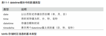
11.1 日期和时间数据类型及工具
一般使用datetime.datetime数据类型。
from datetime import datetime
now= datetime.now()
print(now)
print(now.year,now.month,now.day)
#datetime是用毫秒的方式存储时间的
2020-02-05 11:59:28.917677
2020 2 5
delta = datetime(2011, 1, 7) - datetime(2008, 6, 24, 8, 15)

print(delta.days)
print('\n')
print(delta.seconds)

print('\n')
print(delta)#delta是一个timedelta对象,表示两个datetime对象之间的时间差。
926


56700


926 days, 15:45:00
可以给datetime加上或减去一个或者多个timedelta。
from datetime import timedelta
start = datetime(2011, 1, 7)
start + timedelta(12)
start - 2 * timedelta(12)
datetime.datetime(2010, 12, 14, 0, 0)
字符串和datetime的相互转换
利用str或strftime方法可以将datetime对象和pandas的timestamp对象转化挖诶字符串。
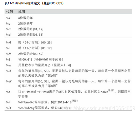
datetime的strftime方法可以对把上述格式的编码字符串转换为日期。
stamp = datetime(2011, 1, 3)
print(str(stamp))
print(stamp.strftime('%Y-%m-%d'))
2011-01-03 00:00:00
2011-01-03
value = '2011-01-03'
datetime.strptime(value, '%Y-%m-%d')
datestrs = ['7/6/2011', '8/6/2011']
print([datetime.strptime(x, '%m/%d/%Y') for x in datestrs])
[datetime.datetime(2011, 7, 6, 0, 0), datetime.datetime(2011, 8, 6, 0, 0)]
对于常用的日期格式,可以用dateutil这个第三方包中的parser.parse方法。
from dateutil.parser import parse
parse('2011-01-03')
parse('Jan 31, 1997 10:45 PM')
datetime.datetime(1997, 1, 31, 22, 45)
#日出现在月的前面很普遍,传入dayfirst=True即可解决这个问题:
parse('6/12/2011', dayfirst=True)
datetime.datetime(2011, 12, 6, 0, 0)
import pandas as pd
#to_datetime方法可以解析多种不同的日期表示形式
datestrs = ['2011-07-06 12:00:00', '2011-08-06 00:00:00']
pd.to_datetime(datestrs)
DatetimeIndex(['2011-07-06 12:00:00', '2011-08-06 00:00:00'], dtype='datetime64[ns]', freq=None)
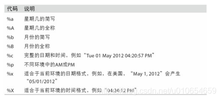
特定于当前环境的日期格式。
11.2 时间序列基础
from datetime import datetime
import numpy as np
dates = [datetime(2011, 1, 2), datetime(2011, 1, 5),
         datetime(2011, 1, 7), datetime(2011, 1, 8),
         datetime(2011, 1, 10), datetime(2011, 1, 12)]
ts = pd.Series(np.random.randn(6), index=dates)
print(ts)
2011-01-02   -1.716667
2011-01-05   -1.539430
2011-01-07   -1.207904
2011-01-08   -2.273456
2011-01-10    0.205142
2011-01-12    0.316390
dtype: float64
ts.index
DatetimeIndex(['2011-01-02', '2011-01-05', '2011-01-07', '2011-01-08',
               '2011-01-10', '2011-01-12'],
              dtype='datetime64[ns]', freq=None)
ts + ts[::2]
2011-01-02   -3.433335
2011-01-05         NaN
2011-01-07   -2.415809
2011-01-08         NaN
2011-01-10    0.410284
2011-01-12         NaN
dtype: float64
ts.index.dtype
dtype('<M8[ns]')
stamp = ts.index[0]
stamp
Timestamp('2011-01-02 00:00:00')
索引、选取、子集构造
stamp = ts.index[2]
ts[stamp]
-1.2079043608040851
#还可以传入可以被解释成日期的字符串,通过这样的方式,也可以索引数据。
ts['1/10/2011']
0.2051420361141498
#对于长序列,只需要传入“年”或者“年月”即可轻松选取数据的切片。
longer_ts = pd.Series(np.random.randn(1000),
                      index=pd.date_range('1/1/2000', periods=1000))
print(longer_ts['2001'])#选择年
print('\n')
print(longer_ts['2001-05'])#选择年月
2001-01-01    0.338687
2001-01-02   -1.073274
2001-01-03    0.637883
2001-01-04    0.309464
2001-01-05    0.692688
                ...
2001-12-27    0.264949
2001-12-28    0.881644
2001-12-29   -2.017786
2001-12-30    0.003661
2001-12-31   -0.060487
Freq: D, Length: 365, dtype: float64


2001-05-01    0.936911
2001-05-02    1.060100
2001-05-03    0.044787
2001-05-04   -0.780111
2001-05-05   -2.865649
2001-05-06   -1.078818
2001-05-07   -1.159225
2001-05-08   -0.327021
2001-05-09   -0.410140
2001-05-10   -0.851768
2001-05-11    0.519780
2001-05-12   -0.236362
2001-05-13    2.319194
2001-05-14   -1.141007
2001-05-15   -0.348985
2001-05-16   -0.118603
2001-05-17   -0.049692
2001-05-18   -0.210484
2001-05-19    0.804600
2001-05-20   -0.697858
2001-05-21   -0.275231
2001-05-22    1.777904
2001-05-23    1.053514
2001-05-24   -2.172931
2001-05-25    0.509915
2001-05-26    0.926985
2001-05-27    1.499682
2001-05-28    0.007916
2001-05-29    1.339204
2001-05-30    1.239413
2001-05-31   -1.425689
Freq: D, dtype: float64
#datetime对象也可以切片.方式是通过将时间作为索引。
ts[datetime(2011, 1, 7):]
2011-01-07   -1.207904
2011-01-08   -2.273456
2011-01-10    0.205142
2011-01-12    0.316390
dtype: float64
ts['1/6/2011':'1/11/2011']
2011-01-07   -1.207904
2011-01-08   -2.273456
2011-01-10    0.205142
dtype: float64
带有重复索引的时间序列
dates = pd.DatetimeIndex(['1/1/2000', '1/2/2000', '1/2/2000',
                          '1/2/2000', '1/3/2000'])
dup_ts = pd.Series(np.arange(5), index=dates)
print(dup_ts)
2000-01-01    0
2000-01-02    1
2000-01-02    2
2000-01-02    3
2000-01-03    4
dtype: int32
#通过is_unique属性,可以判断时间序列数据的索引是不是唯一的
dup_ts.index.is_unique
False
#如果要对非唯一的时间戳的数据进行聚合,可以使用groupby,对level设置为0.
grouped = dup_ts.groupby(level=0)
print(grouped.mean())
print('\n')
print(grouped.count())
2000-01-01    0
2000-01-02    2
2000-01-03    4
dtype: int32


2000-01-01    1
2000-01-02    3
2000-01-03    1
dtype: int64
11.3 日期的范围、频率以及移动
可以将之前那个时间序列转换为1个具有固定频率(每天)的时间序列,只需调用resample即可。
ts
2011-01-02   -1.716667
2011-01-05   -1.539430
2011-01-07   -1.207904
2011-01-08   -2.273456
2011-01-10    0.205142
2011-01-12    0.316390
dtype: float64
resampler = ts.resample('D')#D为每天的意思
生成日期范围
date_range可以生成时间范围。
index = pd.date_range('2012-04-01', '2012-06-01')
print(index)
DatetimeIndex(['2012-04-01', '2012-04-02', '2012-04-03', '2012-04-04',
               '2012-04-05', '2012-04-06', '2012-04-07', '2012-04-08',
               '2012-04-09', '2012-04-10', '2012-04-11', '2012-04-12',
               '2012-04-13', '2012-04-14', '2012-04-15', '2012-04-16',
               '2012-04-17', '2012-04-18', '2012-04-19', '2012-04-20',
               '2012-04-21', '2012-04-22', '2012-04-23', '2012-04-24',
               '2012-04-25', '2012-04-26', '2012-04-27', '2012-04-28',
               '2012-04-29', '2012-04-30', '2012-05-01', '2012-05-02',
               '2012-05-03', '2012-05-04', '2012-05-05', '2012-05-06',
               '2012-05-07', '2012-05-08', '2012-05-09', '2012-05-10',
               '2012-05-11', '2012-05-12', '2012-05-13', '2012-05-14',
               '2012-05-15', '2012-05-16', '2012-05-17', '2012-05-18',
               '2012-05-19', '2012-05-20', '2012-05-21', '2012-05-22',
               '2012-05-23', '2012-05-24', '2012-05-25', '2012-05-26',
               '2012-05-27', '2012-05-28', '2012-05-29', '2012-05-30',
               '2012-05-31', '2012-06-01'],
              dtype='datetime64[ns]', freq='D')
#此外还可以传入时间结束或者开始点
print(pd.date_range(start='2012-04-01', periods=20))
print('\n')
print(pd.date_range(end='2012-06-01', periods=20))
DatetimeIndex(['2012-04-01', '2012-04-02', '2012-04-03', '2012-04-04',
               '2012-04-05', '2012-04-06', '2012-04-07', '2012-04-08',
               '2012-04-09', '2012-04-10', '2012-04-11', '2012-04-12',
               '2012-04-13', '2012-04-14', '2012-04-15', '2012-04-16',
               '2012-04-17', '2012-04-18', '2012-04-19', '2012-04-20'],
              dtype='datetime64[ns]', freq='D')


DatetimeIndex(['2012-05-13', '2012-05-14', '2012-05-15', '2012-05-16',
               '2012-05-17', '2012-05-18', '2012-05-19', '2012-05-20',
               '2012-05-21', '2012-05-22', '2012-05-23', '2012-05-24',
               '2012-05-25', '2012-05-26', '2012-05-27', '2012-05-28',
               '2012-05-29', '2012-05-30', '2012-05-31', '2012-06-01'],
              dtype='datetime64[ns]', freq='D')
按着时间频率进行时间序列的排列
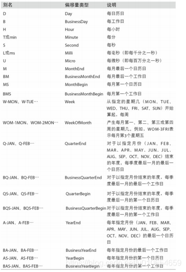
基本的时间序列函数有:
pd.date_range('2000-01-01', '2000-12-01', freq='BM')
#BM表示每月最后一个工作日
DatetimeIndex(['2000-01-31', '2000-02-29', '2000-03-31', '2000-04-28',
               '2000-05-31', '2000-06-30', '2000-07-31', '2000-08-31',
               '2000-09-29', '2000-10-31', '2000-11-30'],
              dtype='datetime64[ns]', freq='BM')
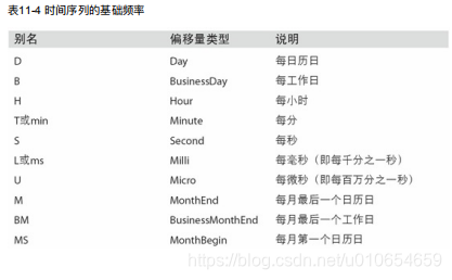
频率和日期偏移量
按着某个频率进行时间上的选取。
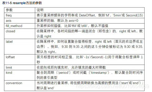
相关的选择参数:

from pandas.tseries.offsets import Hour, Minute


pd.date_range('2000-01-01', '2000-01-03 23:59', freq='4h')
#4个小时选择一次数据
DatetimeIndex(['2000-01-01 00:00:00', '2000-01-01 04:00:00',
               '2000-01-01 08:00:00', '2000-01-01 12:00:00',
               '2000-01-01 16:00:00', '2000-01-01 20:00:00',
               '2000-01-02 00:00:00', '2000-01-02 04:00:00',
               '2000-01-02 08:00:00', '2000-01-02 12:00:00',
               '2000-01-02 16:00:00', '2000-01-02 20:00:00',
               '2000-01-03 00:00:00', '2000-01-03 04:00:00',
               '2000-01-03 08:00:00', '2000-01-03 12:00:00',
               '2000-01-03 16:00:00', '2000-01-03 20:00:00'],
              dtype='datetime64[ns]', freq='4H')
pd.date_range('2000-01-01', periods=10, freq='1h30min')
#每隔1小时30分钟进行数据提取
DatetimeIndex(['2000-01-01 00:00:00', '2000-01-01 01:30:00',
               '2000-01-01 03:00:00', '2000-01-01 04:30:00',
               '2000-01-01 06:00:00', '2000-01-01 07:30:00',
               '2000-01-01 09:00:00', '2000-01-01 10:30:00',
               '2000-01-01 12:00:00', '2000-01-01 13:30:00'],
              dtype='datetime64[ns]', freq='90T')
WOM日期
wom是week of month。
'WOM-3FRI’表示每个月第三个星期五。
移动(超前和滞后)数据
Series和DataFrame都有1个shift方法用于执行单纯的前移或后移操作,保持索引不变。
ts = pd.Series(np.random.randn(4),
               index=pd.date_range('1/1/2000', periods=4, freq='M'))
print(ts)
print('\n')
print(ts.shift(2))
print('\n')
print(ts.shift(-2))
2000-01-31   -0.293180
2000-02-29   -0.593455
2000-03-31   -0.446006
2000-04-30   -0.811115
Freq: M, dtype: float64


2000-01-31         NaN
2000-02-29         NaN
2000-03-31   -0.293180
2000-04-30   -0.593455
Freq: M, dtype: float64


2000-01-31   -0.446006
2000-02-29   -0.811115
2000-03-31         NaN
2000-04-30         NaN
Freq: M, dtype: float64
ts / ts.shift(1) - 1
#可以表示一个时间序列或者多个时间序列中的百分比变化
2000-01-31         NaN
2000-02-29    1.024202
2000-03-31   -0.248458
2000-04-30    0.818619
Freq: M, dtype: float64
通过偏移量对日期进行位移
from pandas.tseries.offsets import Day, MonthEnd
now = datetime(2011, 11, 17)
now + 3 * Day()
Timestamp('2011-11-20 00:00:00')
now + MonthEnd()#时间会到now时间表示的这个月底
Timestamp('2011-11-30 00:00:00')
11.4 时区处理
import pytz
pytz.common_timezones[-5:]
['US/Eastern', 'US/Hawaii', 'US/Mountain', 'US/Pacific', 'UTC']
时区本地化和转换
rng = pd.date_range('3/9/2012 9:30', periods=6, freq='D')
ts = pd.Series(np.random.randn(len(rng)), index=rng)
print(ts)
2012-03-09 09:30:00   -0.736406
2012-03-10 09:30:00   -1.689875
2012-03-11 09:30:00    1.190183
2012-03-12 09:30:00    0.674204
2012-03-13 09:30:00    0.373736
2012-03-14 09:30:00    0.471685
Freq: D, dtype: float64
pd.date_range('3/9/2012 9:30', periods=10, freq='D', tz='UTC')
DatetimeIndex(['2012-03-09 09:30:00+00:00', '2012-03-10 09:30:00+00:00',
               '2012-03-11 09:30:00+00:00', '2012-03-12 09:30:00+00:00',
               '2012-03-13 09:30:00+00:00', '2012-03-14 09:30:00+00:00',
               '2012-03-15 09:30:00+00:00', '2012-03-16 09:30:00+00:00',
               '2012-03-17 09:30:00+00:00', '2012-03-18 09:30:00+00:00'],
              dtype='datetime64[ns, UTC]', freq='D')
#通过tz_localize方法处理时间的本地化转换
ts_utc = ts.tz_localize('UTC')
#当时间转换到某个特定时区后,可以用tz_convent将其转换到其他时区中。
ts_utc.tz_convert('America/New_York')
2012-03-09 04:30:00-05:00   -0.736406
2012-03-10 04:30:00-05:00   -1.689875
2012-03-11 05:30:00-04:00    1.190183
2012-03-12 05:30:00-04:00    0.674204
2012-03-13 05:30:00-04:00    0.373736
2012-03-14 05:30:00-04:00    0.471685
Freq: D, dtype: float64
11.5 时期及其算术
时期的频率转换
Period和PeriodIndex对象都可以通过其asfreq方法被转换成别的频率.
p = pd.Period(2007, freq='A-DEC')
p+5
Period('2012', 'A-DEC')
p.asfreq('M', how='start')#转换为月的数据
Period('2007-01', 'M')
p.asfreq('M', how='end')
Period('2007-12', 'M')
rng = pd.period_range('2006', '2009', freq='A-DEC')
ts = pd.Series(np.random.randn(len(rng)), index=rng)
ts.asfreq('M', how='start')
2006-01    0.295788
2007-01    1.363306
2008-01    1.014115
2009-01   -0.556755
Freq: M, dtype: float64
按季度计算的时期频率
p = pd.Period('2012Q4', freq='Q-JAN')
#注意不同的freq参数,最后确定的数据也是不一样的
p.asfreq('D', 'start')
Period('2011-11-01', 'D')
rng = pd.period_range('2011Q3', '2012Q4', freq='Q-JAN')
ts = pd.Series(np.arange(len(rng)), index=rng)
print(ts)
2011Q3    0
2011Q4    1
2012Q1    2
2012Q2    3
2012Q3    4
2012Q4    5
Freq: Q-JAN, dtype: int32
将Timestamp转换为Period(及其反向过程)
rng = pd.date_range('2000-01-01', periods=3, freq='M')
ts = pd.Series(np.random.randn(3), index=rng)
pts = ts.to_period()
print(ts)
print('\n')
print(pts)
2000-01-31    1.730324
2000-02-29    0.947510
2000-03-31    1.073048
Freq: M, dtype: float64


2000-01    1.730324
2000-02    0.947510
2000-03    1.073048
Freq: M, dtype: float64
通过数组创建PeriodIndex
data = pd.read_csv('examples/macrodata.csv')
print(data.head(5))
     year  quarter   realgdp  realcons  realinv  realgovt  realdpi    cpi  \
0  1959.0      1.0  2710.349    1707.4  286.898   470.045   1886.9  28.98
1  1959.0      2.0  2778.801    1733.7  310.859   481.301   1919.7  29.15
2  1959.0      3.0  2775.488    1751.8  289.226   491.260   1916.4  29.35
3  1959.0      4.0  2785.204    1753.7  299.356   484.052   1931.3  29.37
4  1960.0      1.0  2847.699    1770.5  331.722   462.199   1955.5  29.54

      m1  tbilrate  unemp      pop  infl  realint
0  139.7      2.82    5.8  177.146  0.00     0.00
1  141.7      3.08    5.1  177.830  2.34     0.74
2  140.5      3.82    5.3  178.657  2.74     1.09
3  140.0      4.33    5.6  179.386  0.27     4.06
4  139.6      3.50    5.2  180.007  2.31     1.19
print(data.year)
0      1959.0
1      1959.0
2      1959.0
3      1959.0
4      1960.0
        ...
198    2008.0
199    2008.0
200    2009.0
201    2009.0
202    2009.0
Name: year, Length: 203, dtype: float64
index = pd.PeriodIndex(year=data.year, quarter=data.quarter,
                       freq='Q-DEC')
data.index = index
print(data.infl)
1959Q1    0.00
1959Q2    2.34
1959Q3    2.74
1959Q4    0.27
1960Q1    2.31
          ...
2008Q3   -3.16
2008Q4   -8.79
2009Q1    0.94
2009Q2    3.37
2009Q3    3.56
Freq: Q-DEC, Name: infl, Length: 203, dtype: float64
11.6 重采样及频率转换
高频到低频是降采样,低频到高频是升采样。
rng = pd.date_range('2000-01-01', periods=100, freq='D')
ts = pd.Series(np.random.randn(len(rng)), index=rng)
print(ts)
2000-01-01   -2.036950
2000-01-02    0.196854
2000-01-03    0.191711
2000-01-04    1.131291
2000-01-05    0.225399
                ...
2000-04-05    0.191335
2000-04-06   -1.054301
2000-04-07    0.571078
2000-04-08    0.314156
2000-04-09   -0.375186
Freq: D, Length: 100, dtype: float64
ts.resample('M').mean()
2000-01-31    0.071255
2000-02-29   -0.007097
2000-03-31    0.019090
2000-04-30    0.266123
Freq: M, dtype: float64
#降采样
rng = pd.date_range('2000-01-01', periods=12, freq='T')
ts = pd.Series(np.arange(12), index=rng)
print(ts)
2000-01-01 00:00:00     0
2000-01-01 00:01:00     1
2000-01-01 00:02:00     2
2000-01-01 00:03:00     3
2000-01-01 00:04:00     4
2000-01-01 00:05:00     5
2000-01-01 00:06:00     6
2000-01-01 00:07:00     7
2000-01-01 00:08:00     8
2000-01-01 00:09:00     9
2000-01-01 00:10:00    10
2000-01-01 00:11:00    11
Freq: T, dtype: int32
ts.resample('5min', closed='right').sum()
#默认情况下,面元的右边界是包含的,因此00:00到00:05的区间中是包含00:05的。
1999-12-31 23:55:00     0
2000-01-01 00:00:00    15
2000-01-01 00:05:00    40
2000-01-01 00:10:00    11
Freq: 5T, dtype: int32
OHLC重采样
第一个值、最后一个值、最大值、最小值。传入how='chlc’即可。
print(ts.resample('5min').ohlc())
                     open  high  low  close
2000-01-01 00:00:00     0     4    0      4
2000-01-01 00:05:00     5     9    5      9
2000-01-01 00:10:00    10    11   10     11
升采样和插值
frame = pd.DataFrame(np.random.randn(2, 4),
                     index=pd.date_range('1/1/2000', periods=2,
                                         freq='W-WED'),
                     columns=['Colorado', 'Texas', 'New York', 'Ohio'])
df_daily = frame.resample('D').asfreq()
print(df_daily)
            Colorado     Texas  New York      Ohio
2000-01-05 -0.141497 -0.299701  0.374013 -1.185863
2000-01-06       NaN       NaN       NaN       NaN
2000-01-07       NaN       NaN       NaN       NaN
2000-01-08       NaN       NaN       NaN       NaN
2000-01-09       NaN       NaN       NaN       NaN
2000-01-10       NaN       NaN       NaN       NaN
2000-01-11       NaN       NaN       NaN       NaN
2000-01-12  0.396594 -0.509955  1.038497  2.786482
11.7 移动窗口函数
import matplotlib.pyplot as plt
close_px_all = pd.read_csv('examples/stock_px_2.csv',
                           parse_dates=True, index_col=0)
close_px = close_px_all[['AAPL', 'MSFT', 'XOM']]
close_px = close_px.resample('B').ffill()
close_px.AAPL.plot()
close_px.AAPL.rolling(250).mean().plot()
<matplotlib.axes._subplots.AxesSubplot at 0x92ce330>
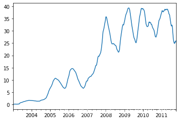
appl_std250 = close_px.AAPL.rolling(250, min_periods=10).std()
appl_std250.plot()
<matplotlib.axes._subplots.AxesSubplot at 0x937d6f0>
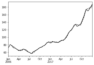
指数加权函数
aapl_px = close_px.AAPL['2006':'2007']
ma60 = aapl_px.rolling(30, min_periods=20).mean()
ewma60 = aapl_px.ewm(span=30).mean()
ma60.plot(style='k--', label='Simple MA')
ewma60.plot(style='k-', label='EW MA')
<matplotlib.axes._subplots.AxesSubplot at 0x95491f0>
说明:
放上参考链接,复现的这个链接中的内容。
放上原链接: https://www.jianshu.com/p/04d180d90a3f
作者在链接中放上了书籍,以及相关资源。因为平时杂七杂八的也学了一些,所以这次可能是对书中的部分内容的复现。也可能有我自己想到的内容,内容暂时都还不定。在此感谢原简书作者SeanCheney的分享


 344
344


 被折叠的 条评论
为什么被折叠?
被折叠的 条评论
为什么被折叠?
 到【灌水乐园】发言


