


一、一元线性回归
一元线性回归:一个响应变量和一个解释变量的一元问题。
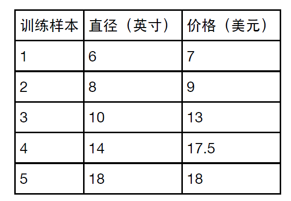
1.分析匹萨的直径与价格的数据的线性关系,数据如下
2. 根据样本绘制散点图:
程序:
defrunplt():
plt.figure()
plt.title('匹萨价格与直径数据',fontproperties=font)
plt.xlabel('直径(英寸)',fontproperties=font)
plt.ylabel('价格(美元)',fontproperties=font)
plt.axis([0,25,0,25])
plt.grid(True)
returnplt
import matplotlib.pyplotasplt
from matplotlib.font_managerimportFontProperties
font = FontProperties(fname=r"c:\windows\fonts\msyh.ttc",size=10)
plt = runplt()
X = [[6],[8],[10],[14],[18]]
y = [[7],[9],[13],[17.5],[18]]
plt.plot(X,y,'k.')
plt.show()
Python2.7会报如下错误:
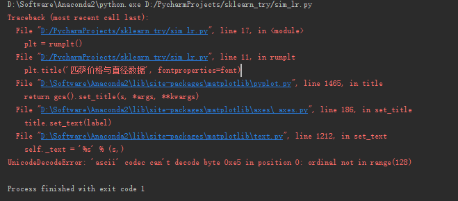
解决方案,在import前加上下面三行即可
importsys
reload(sys)
sys.setdefaultencoding('utf-8')
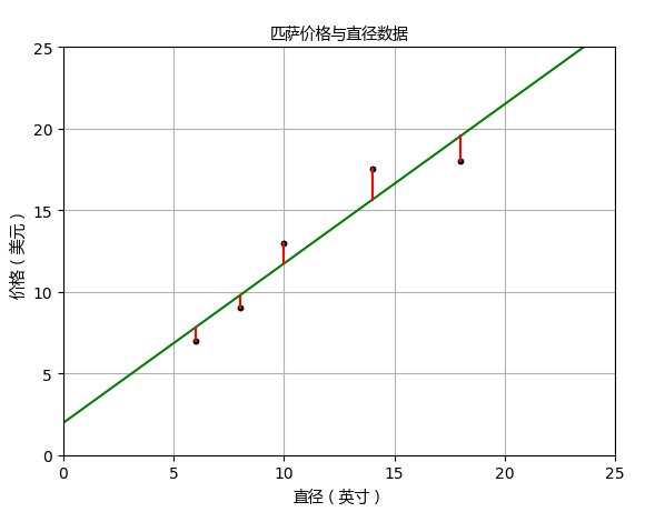
3、用scikit-learn来构建模型
程序:
from sklearn.linear_modelimport LinearRegression
# 创建并拟合模型
X = [[6],[8],[10],[14],[18]]
y = [[7],[9],[13],[17.5],[18]]
model = LinearRegression()
model.fit(X,y)
print('预测一张12英寸匹萨价格:$%.2f'% model.predict([[12]])[0])
plt = runplt()
plt.plot(X,y,'k.')
X2 = [[0],[10],[14],[25]]
y2 = model.predict(X2)
plt.plot(X2,y2,'g-')
# 残差预测值
yr = model.predict(X)
for idx,xinenumerate(X):
plt.plot([x,x],[y[idx],yr[idx]],'r-')
plt.show()
上述代码中sklearn.linear_model.LinearRegression类是一个估计器(estimator)。在scikit-learn里面,所有的估计器都带有fit()和predict()方法。fit()用来分析模型参数,predict()是通过fit()算出的模型参数构成的模型,对解释变量进行预测获得的值。LinearRegression类的fit()方法学习下面的一元线性回归模型:

一元线性回归拟合模型的参数估计常用方法是普通最小二乘法(ordinary least squares )或线性最小二乘法(linear least squares)。成本函数(cost function)也叫损失函数(loss function),用来定义模型与观测值的误差。
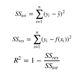
3、模型评估
R方也叫确定系数(coefficient of determination),表示模型对现实数据拟合的程度。
加入模型评估程序
X_test = [[8],[9],[11],[16],[12]]
y_test = [[11],[8.5],[15],[18],[11]]
model = LinearRegression()
model.fit(X,y)
print model.score(X_test,y_test)
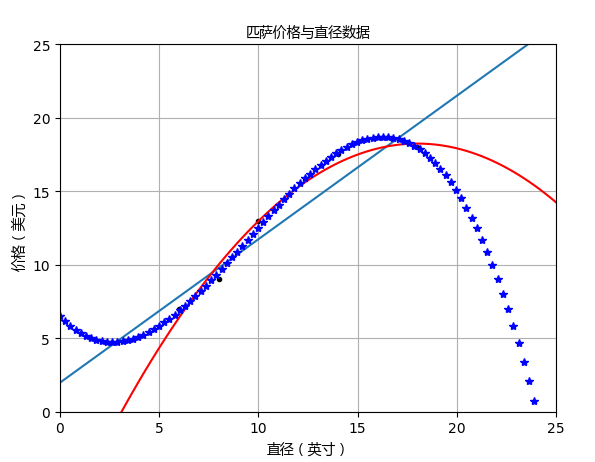
二、多项式回归

PolynomialFeatures转换器可以用来解决多项式回归问题
程序:
importnumpyasnp
from sklearn.linear_modelimportLinearRegression
from sklearn.preprocessingimportPolynomialFeatures
X_train = [[6],[8],[10],[14],[18]]
y_train = [[7],[9],[13],[17.5],[18]]
X_test = [[6],[8],[11],[16]]
y_test = [[8],[12],[15],[18]]
regressor = LinearRegression()
regressor.fit(X_train,y_train)
xx = np.linspace(0,26,100)
yy = regressor.predict(xx.reshape(xx.shape[0],1))
plt = runplt()
plt.plot(X_train,y_train,'k.')
plt.plot(xx,yy)
quadratic_featurizer = PolynomialFeatures(degree=2)
X_train_quadratic = quadratic_featurizer.fit_transform(X_train)
X_test_quadratic = quadratic_featurizer.transform(X_test)
regressor_quadratic = LinearRegression()
regressor_quadratic.fit(X_train_quadratic,y_train)
xx_quadratic = quadratic_featurizer.transform(xx.reshape(xx.shape[0],1))
plt.plot(xx,regressor_quadratic.predict(xx_quadratic),'r-')
cubic_featurizer = PolynomialFeatures(degree=3)
X_train_cubic = cubic_featurizer.fit_transform(X_train)
X_test_cubic = cubic_featurizer.transform(X_test)
regressor_cubic = LinearRegression()
regressor_cubic.fit(X_train_cubic,y_train)
xx_cubic = cubic_featurizer.transform(xx.reshape(xx.shape[0],1))
plt.plot(xx,regressor_cubic.predict(xx_cubic),'b*')
plt.show()
print("一元线性回归 r-squared:%.2f"%(regressor.score(X_test,y_test)))
print("二次回归 r-squared:%.2f"%(regressor_quadratic.score(X_test_quadratic,y_test)))
print("二次回归 r-squared:%.2f"%(regressor_cubic.score(X_test_cubic ,y_test)))
运行结果:
三、多元线性回归

训练样本:
X = [[6, 2], [8, 1], [10, 0], [14, 2], [18, 0]]
y = [[7], [9], [13], [17.5], [18]]
测试样本:
X_test = [[8, 2], [9, 0], [11, 2], [16, 2], [12, 0]]
y_test = [[11], [8.5], [15], [18], [11]]
程序:
fromsklearn.linear_modelimport LinearRegression
X = [[6,2],[8,1],[10,0],[14,2],[18,0]]
y = [[7],[9],[13],[17.5],[18]]
model = LinearRegression()
model.fit(X,y)
X_test = [[8,2],[9,0],[11,2],[16,2],[12,0]]
y_test = [[11],[8.5],[15],[18],[11]]
predictions = model.predict(X_test)
for i,predictioninenumerate(predictions):
print('Predicted: %s, Target: %s'% (prediction,y_test[i]))
print('R-squared: %.2f'% model.score(X_test,y_test))
运行结果:


 4万+
4万+

 被折叠的 条评论
为什么被折叠?
被折叠的 条评论
为什么被折叠?
 到【灌水乐园】发言


