逻辑回归-梯度下降法 python实现

机器学习的基本框架：

模型(model)、目标(cost function)、优化算法

Step1：对于一个问题，需要首先建立一个模型，如回归或分类模型；

step2：通过最小分类误差、最大似然或最大后验概率建立模型的代价函数；

step3：最优化问题求解

a.如果优化函数存在解析解，则可以通过一般的求值方法-对代价函数求导，找到倒数为0的点，即是最大值或者最小孩子；

b.如果上述方法求优化函数导数比较复杂，可利用迭代算法也求解。

对于回归问题：

（1）模型

可选择的模型有线性回归和LR回归。

（2）目标-cost function

线性回归模型：

 （最小二乘）

LR回归模型：

（极大似然）

线性回归的假设前提是y服从正态分布，LR回归的假设前提是y服从二项分布（y非零即1）。

（3）算法-最优化算法

梯度下降法、牛顿法等；

Python代码：

LRgradAscent.py

from numpy import *

def loadData(filepath):
    dataMat= []
    labels = []
    fr = open(filepath)
    for line in fr.readlines():
        str = line.strip().split('\t')
        dataMat.append([1.0,float(str[0]),float(str[1])])
        labels.append(int(str[2]))
    return mat(dataMat), mat(labels).transpose()

def sigmoid(inX):
    return 1.0/(1+exp(-inX))

def gradAscent(dataMatrix,labelsMatrix):
    n,m = shape(dataMatrix)
    weights = ones((m,1))
    step = 0.001
    iter = 500
    for k in range(iter):
        value = sigmoid(dataMatrix*weights)
        chazhi = labelsMatrix - value
        grad = dataMatrix.transpose()*chazhi
        weights = weights + step * grad
    return weights
    
def plotBestFit(weights,filepath):
    import matplotlib.pyplot as plt
    # illustrate the samples
    dataMatrix,labelsMatrix = loadData(filepath)
    n,m = shape(dataMatrix)
    xcord1 = []; ycord1 = []  #store the coordination of sample having label 1
    xcord2 = []; ycord2 = []
    for i in range(n):
        if int(labelsMatrix[i]) == 1:
            xcord1.append(dataMatrix[i,1])
            ycord1.append(dataMatrix[i,2])
        else:
            xcord2.append(dataMatrix[i,1])
            ycord2.append(dataMatrix[i,2])
    fig = plt.figure()
    ax = fig.add_subplot(111)
    ax.scatter(xcord1,ycord1,s = 30,c = 'red',marker = 's')
    ax.scatter(xcord2,ycord2,s = 30,c = 'green')
    
    #illustrate the classifying line
    min_x = min(dataMatrix[:,1])[0,0]
    max_x = max(dataMatrix[:,2])[0,0]
    y_min_x = (-weights[0] - weights[1] * min_x) / weights[2]
    y_max_x = (-weights[0] - weights[1] * max_x) / weights[2]  #here, sigmoid(wx = 0) so wo + w1*x1 + w2*x2 = 0
    plt.plot([min_x,max_x],[y_min_x[0,0],y_max_x[0,0]],'-g') 
    plt.show()

测试程序：

import LRgradAscent
import pdb

filename = 'testSet.txt'
dataMat, labelsMat = LRgradAscent.loadData(filename)
weights = LRgradAscent.gradAscent(dataMat,labelsMat)
LRgradAscent.plotBestFit(weights,filename)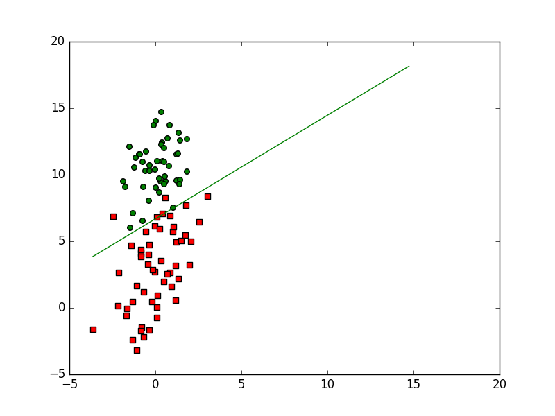

参考：http://blog.csdn.net/zouxy09/article/details/20319673