特征选择是一个重要的数据预处理过程,获得数据之后要先进行特征选择然后再训练模型。主要作用:1、降维 2、去除不相关特征。
特征选择方法包含:子集搜索和子集评价两个问题。
子集搜索包含前向搜索、后向搜索、双向搜索等。
子集评价方法包含:信息增益,交叉熵,相关性,余弦相似度等评级准则。
两者结合起来就是特征选择方法,例如前向搜索与信息熵结合,显然与决策树很相似。
常见特征选择有三类方法:过滤式(filter),包裹式(wrapper)和嵌入式(embedding).————见周志华老师《机器学习》11章。
1. 过滤式(filter)
过滤式方法先对数据集进行特征选择,再训练学习器。两者分裂开来。Relief是一种著名的过滤式特征选择方法,设计了一种相关统计量来度量特征重要性。
sklearn模块中有一些特征选择的方法。
sklearn官方文档
(1)* Removing features with low variance*
特征筛选的时候,对于特征全0,全1 ,多数1,多数0的要删去。利用sklearn中模块,可如下操作(个人认为属于过滤式的)。
代码如下:
from sklearn.feature_selection import VarianceThreshold
 X = [[0, 0, 1], [0, 1, 0], [1, 0, 0], [0, 1, 1], [0, 1, 0], [0, 1, 1]]
sel = VarianceThreshold(threshold=(.8 * (1 - .8))) #选择方差大于某个数的特征。
sel.fit_transform(X)
array([[0, 1],
       [1, 0],
       [0, 0],
       [1, 1],
       [1, 0],
       [1, 1]])
(2)利用单变量特征选择(统计测试方法)。
Univariate feature selection works by selecting the best features based on univariate statistical tests. It can be seen as a preprocessing step to an estimator. Scikit-learn exposes feature selection routines as objects that implement the transform method:
SelectKBest选择排名排在前n个的变量
SelectPercentile 选择排名排在前n%的变量
其他指标: false positive rate SelectFpr, false discovery rate SelectFdr, or family wise error SelectFwe 和 GenericUnivariateSelect。
对于regression问题:用f_regression函数。
对于classification问题:用chi2或者f_classif函数。
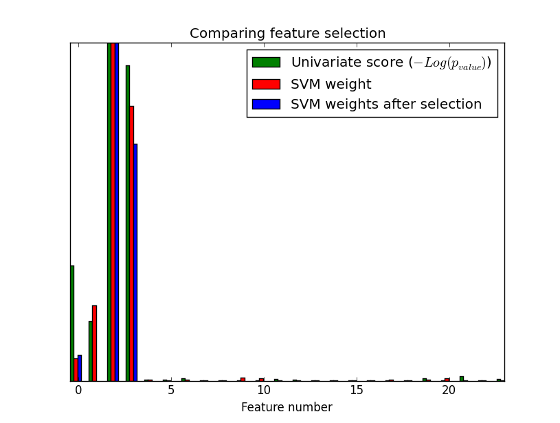
例如:利用 F-test for feature scoring
We use the default selection function: the 10% most significant features**
代码来源
print(__doc__)
import numpy as np
import matplotlib.pyplot as plt
from sklearn import datasets, svm
from sklearn.feature_selection import SelectPercentile, f_classif
iris = datasets.load_iris()
E = np.random.uniform(0, 0.1, size=(len(iris.data), 20))
X = np.hstack((iris.data, E))
print X.shape
y = iris.target
plt.figure(1)
plt.clf()
X_indices = np.arange(X.shape[-1])
selector = SelectPercentile(f_classif, percentile=10)
selector.fit(X, y)
scores = -np.log10(selector.pvalues_)
scores /= scores.max()
plt.bar(X_indices - .45, scores, width=.2,
label=r'Univariate score ($-Log(p_{value})$)', color='g')
clf = svm.SVC(kernel='linear')
clf.fit(X, y)
svm_weights = (clf.coef_ ** 2).sum(axis=0)
svm_weights /= svm_weights.max()
plt.bar(X_indices - .25, svm_weights, width=.2, label='SVM weight', color='r')
clf_selected = svm.SVC(kernel='linear')
clf_selected.fit(selector.transform(X), y)
svm_weights_selected = (clf_selected.coef_ ** 2).sum(axis=0)
svm_weights_selected /= svm_weights_selected.max()
plt.bar(X_indices[selector.get_support()] - .05, svm_weights_selected,
width=.2, label='SVM weights after selection', color='b')
plt.title("Comparing feature selection")
plt.xlabel('Feature number')
plt.yticks(())
plt.axis('tight')
plt.legend(loc='upper right')
plt.show()
- 1
- 2
- 3
- 4
- 5
- 6
- 7
- 8
- 9
- 10
- 11
- 12
- 13
- 14
- 15
- 16
- 17
- 18
- 19
- 20
- 21
- 22
- 23
- 24
- 25
- 26
- 27
- 28
- 29
- 30
- 31
- 32
- 33
- 34
- 35
- 36
- 37
- 38
- 39
- 40
- 41
- 42
- 43
- 44
- 45
- 46
- 47
- 48
- 49
- 50
- 51
- 52
- 53
- 54
- 55
- 56
- 57
- 58
- 59
- 60
- 61
- 62
- 63
- 64
P值越小,显著性越高。负对数也越大。前4个有明显的显著性。(后20个无显著性)
2.包裹式(wrapper)
与过滤式机器学习不考虑后续学习器不同,包裹式特征选择直接把最终要使用的学习器性能作为特征子集的评价标准。由于包裹式特征选择的方法直接针对给定学习器进行优化,包裹式特征一般回避过滤式要好。LVW是一种典型的方法。采用随机策略搜索特征子集,而每次特征子集的评价都需要训练学习器,开销很大。
3.嵌入式(embedding)
嵌入式特征选择将特征选择过程和机器训练过程融合为一体。两者在同一优化过程中完成,即在学习器训练过程中自动进行了特征选择。
例如:L1正则化(Lasso,注意L2岭回归并不会降低维度)
from sklearn.svm import LinearSVC
from sklearn.datasets import load_iris
from sklearn.feature_selection import SelectFromModel
iris = load_iris()
X, y = iris.data, iris.target
X.shape
(150, 4)
lsvc = LinearSVC(C=0.01, penalty="l1", dual=False).fit(X, y)
model = SelectFromModel(lsvc, prefit=True)
X_new = model.transform(X)
X_new.shape
(150, 3)
基于树的特征选取
对于树模型选择特征属于上面哪一种,感觉是包裹式,并不确定。
sklearn 提供例子:
class sklearn.ensemble.ExtraTreesClassifier(n_estimators=10, criterion=’gini’, max_depth=None, min_samples_split=2……)
分类标准 默认基尼系数,还可以设成信息熵增益。
print(__doc__)

import numpy as np
import matplotlib.pyplot as plt

from sklearn.datasets import make_classification
from sklearn.ensemble import ExtraTreesClassifier

# Build a classification task using 3 informative features
X, y = make_classification(n_samples=1000,
                           n_features=10,
                           n_informative=3,
                           n_redundant=0,
                           n_repeated=0,
                           n_classes=2,
                           random_state=0,
                           shuffle=False)

# Build a forest and compute the feature importances
forest = ExtraTreesClassifier(n_estimators=250,
                              random_state=0)
forest.fit(X, y)
importances = forest.feature_importances_
std = np.std([tree.feature_importances_ for tree in forest.estimators_],
             axis=0)
indices = np.argsort(importances)[::-1]

# Print the feature ranking
print("Feature ranking:")

for f in range(X.shape[1]):
    print("%d. feature %d (%f)" % (f + 1, indices[f], importances[indices[f]]))

# Plot the feature importances of the forest
plt.figure()
plt.title("Feature importances")
plt.bar(range(X.shape[1]), importances[indices],
       color="r", yerr=std[indices], align="center")
plt.xticks(range(X.shape[1]), indices)
plt.xlim([-1, X.shape[1]])
plt.show()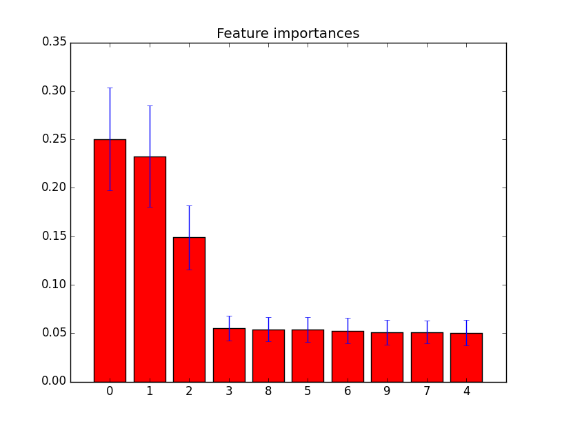


 2万+
2万+

 被折叠的 条评论
为什么被折叠?
被折叠的 条评论
为什么被折叠?
 到【灌水乐园】发言


