opencv（c++）离散傅立叶变换

参考：
1、https://docs.opencv.org/3.2.0/
2、https://github.com/opencv/opencv/

---

Discrete Fourier Transform

• 什么是傅立叶变换，为什么使用它？
• 如何在OpenCV中做到这一点？
• cv :: copyMakeBorder（），cv :: merge（），cv :: dft（），cv ::
  getOptimalDFTSize（），cv :: log（）和cv :: normalize（）函数的使用。

---

源代码

您可以从这里下载，或者在OpenCV源代码库的samples / cpp / tutorial_code / core / discrete_fourier_transform / discrete_fourier_transform.cpp中找到它。

以下是cv :: dft()的一个示例用法：

#include "opencv2/core.hpp"
#include "opencv2/imgproc.hpp"
#include "opencv2/imgcodecs.hpp"
#include "opencv2/highgui.hpp"

#include <iostream>

using namespace cv;
using namespace std;

static void help(void)
{
    cout << endl
        <<  "This program demonstrated the use of the discrete Fourier transform (DFT). " << endl
        <<  "The dft of an image is taken and it's power spectrum is displayed."          << endl
        <<  "Usage:"                                                                      << endl
        <<  "./discrete_fourier_transform [image_name -- default ../data/lena.jpg]"       << endl;
}

int main(int argc, char ** argv)
{
    help();

    const char* filename = argc >=2 ? argv[1] : "../data/lena.jpg";

    Mat I = imread(filename, IMREAD_GRAYSCALE);
    if( I.empty()){
        cout << "Error opening image" << endl;
        return -1;
    }

//! [expand]
    Mat padded;                            //expand input image to optimal size
    int m = getOptimalDFTSize( I.rows );
    int n = getOptimalDFTSize( I.cols ); // on the border add zero values
    copyMakeBorder(I, padded, 0, m - I.rows, 0, n - I.cols, BORDER_CONSTANT, Scalar::all(0));
//! [expand]

//! [complex_and_real]
    Mat planes[] = {Mat_<float>(padded), Mat::zeros(padded.size(), CV_32F)};
    Mat complexI;
    merge(planes, 2, complexI);         // Add to the expanded another plane with zeros
//! [complex_and_real]

//! [dft]
    dft(complexI, complexI);            // this way the result may fit in the source matrix
//! [dft]

    // compute the magnitude and switch to logarithmic scale
    // => log(1 + sqrt(Re(DFT(I))^2 + Im(DFT(I))^2))
//! [magnitude]
    split(complexI, planes);                   // planes[0] = Re(DFT(I), planes[1] = Im(DFT(I))
    magnitude(planes[0], planes[1], planes[0]);// planes[0] = magnitude
    Mat magI = planes[0];
//! [magnitude]

//! [log]
    magI += Scalar::all(1);                    // switch to logarithmic scale
    log(magI, magI);
//! [log]

//! [crop_rearrange]
    // crop the spectrum, if it has an odd number of rows or columns
    magI = magI(Rect(0, 0, magI.cols & -2, magI.rows & -2));

    // rearrange the quadrants of Fourier image  so that the origin is at the image center
    int cx = magI.cols/2;
    int cy = magI.rows/2;

    Mat q0(magI, Rect(0, 0, cx, cy));   // Top-Left - Create a ROI per quadrant
    Mat q1(magI, Rect(cx, 0, cx, cy));  // Top-Right
    Mat q2(magI, Rect(0, cy, cx, cy));  // Bottom-Left
    Mat q3(magI, Rect(cx, cy, cx, cy)); // Bottom-Right

    Mat tmp;                           // swap quadrants (Top-Left with Bottom-Right)
    q0.copyTo(tmp);
    q3.copyTo(q0);
    tmp.copyTo(q3);

    q1.copyTo(tmp);                    // swap quadrant (Top-Right with Bottom-Left)
    q2.copyTo(q1);
    tmp.copyTo(q2);
//! [crop_rearrange]

//! [normalize]
    normalize(magI, magI, 0, 1, NORM_MINMAX); // Transform the matrix with float values into a
                                            // viewable image form (float between values 0 and 1).
//! [normalize]

    imshow("Input Image"       , I   );    // Show the result
    imshow("spectrum magnitude", magI);
    waitKey();

    return 0;
}

---

说明

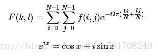
傅立叶变换将图像分解为其正弦和余弦分量。 换句话说，它会将图像从其空间域转换到其频域。 这个想法是任何函数都可以用无限的正弦函数和余弦函数的和来逼近。 傅立叶变换是一种如何做到这一点的方法。 在数学上二维图像傅里叶变换是：

这里$f$是在其空间域中的图像值和在其频域中的$F$。 转换的结果是复数。 通过真实的图像和复杂的图像或通过幅度和相位图像来显示这个是可能的。 然而，在整个图像处理算法中，只有幅度图像是有趣的，因为这包含了我们所需要的关于图像几何结构的所有信息。 不过，如果你打算对这些形式的图像进行一些修改，然后你需要重新形成它，你需要保留这两个。

在这个例子中，我将展示如何计算和显示傅立叶变换的幅度图像。 在数字图像是离散的情况下。 这意味着他们可能会从一个给定的域值中获得一个值。 例如，在基本灰度级中，图像值通常在0和255之间。因此，傅立叶变换也需要是离散型的，导致离散傅里叶变换（DFT）。 每当需要从几何角度确定图像的结构时，您都会希望使用它。 以下是要遵循的步骤（如果是灰度输入图像$I$）：

1、将图像展开至最佳尺寸。 DFT的性能取决于图像大小。 对于二，三，五倍的图像尺寸来说，它往往是最快的。 因此，为了获得最佳性能，通常将边界值填充到图像以获得具有这种特性的大小是一个好主意。 cv :: getOptimalDFTSize（）返回这个最佳尺寸，我们可以使用cv :: copyMakeBorder（）函数来展开图像的边界：

Mat padded;                            //expand input image to optimal size
int m = getOptimalDFTSize( I.rows );
int n = getOptimalDFTSize( I.cols ); // on the border add zero pixels
copyMakeBorder(I, padded, 0, m - I.rows, 0, n - I.cols, BORDER_CONSTANT, Scalar::all(0));

附加像素初始化为零。

2、为复数和实际数值做好准备。 傅里叶变换的结果是复数。 这意味着对于每个图像值，结果是两个图像值（每个分量一个）。 而且，频域范围远大于空间范围。 因此，我们通常至少以浮点格式存储这些数据。 因此，我们将把输入图像转换为这种类型，并用另一个通道来扩展它以保存复杂的值：

Mat planes[] = {Mat_<float>(padded), Mat::zeros(padded.size(), CV_32F)};
Mat complexI;
merge(planes, 2, complexI);         // Add to the expanded another plane with zeros

3、进行离散傅里叶变换。 有可能in-place计算（与输出相同的输入）：

dft(complexI, complexI);            // this way the result may fit in the source matrix

4、将真实的和复数的值转化为数值。 一个复数有一个实数（Re）和一个复数（虚数 - Im）的部分。 DFT的结果是复数。 DFT的大小是：
$M$ = $\sqrt[2]{ {Re(DFT(I))}^2 + {Im(DFT(I))}^2}$

转换为OpenCV代码：

split(complexI, planes);                   // planes[0] = Re(DFT(I), planes[1] = Im(DFT(I))
magnitude(planes[0], planes[1], planes[0]);// planes[0] = magnitude
Mat magI = planes[0];

5、切换到对数刻度。 事实证明，傅立叶系数的动态范围太大而不能显示在屏幕上。 我们有一些小而高的变化值，我们不能这样观察。 因此，高值将全部变成白点，而小值变成黑色。 要使用灰度值进行可视化，我们可以将线性比例转换为对数：
$M_1$ = $\log{(1 + M)}$

转换为OpenCV代码：

magI += Scalar::all(1);                    // switch to logarithmic scale
log(magI, magI);

6、裁剪和重新排列。 请记住，在第一步，我们扩大了形象？ 那么，现在是时候扔掉新引入的值。 为了可视化的目的，我们还可以重新排列结果的象限，使得原点（零点，零点）与图像中心相对应。

magI = magI(Rect(0, 0, magI.cols & -2, magI.rows & -2));
int cx = magI.cols/2;
int cy = magI.rows/2;
Mat q0(magI, Rect(0, 0, cx, cy));   // Top-Left - Create a ROI per quadrant
Mat q1(magI, Rect(cx, 0, cx, cy));  // Top-Right
Mat q2(magI, Rect(0, cy, cx, cy));  // Bottom-Left
Mat q3(magI, Rect(cx, cy, cx, cy)); // Bottom-Right
Mat tmp;                           // swap quadrants (Top-Left with Bottom-Right)
q0.copyTo(tmp);
q3.copyTo(q0);
tmp.copyTo(q3);
q1.copyTo(tmp);                    // swap quadrant (Top-Right with Bottom-Left)
q2.copyTo(q1);
tmp.copyTo(q2);

7、规范化。 为了可视化的目的，这再次完成。 我们现在有了这些幅度，但是这仍然超出了从零到一的图像显示范围。 我们使用cv :: normalize（）函数将我们的值规范化到这个范围。

normalize(magI, magI, 0, 1, NORM_MINMAX); // Transform the matrix with float values into a
                                          // viewable image form (float between values 0 and 1).