基于内容推荐系统_基于内容的推荐系统-CSDN博客

本文深入探讨了基于内容的推荐系统，介绍了其工作原理和实现方式，涵盖了从数据处理到模型构建的关键步骤。

摘要由CSDN通过智能技术生成

基于内容推荐系统

介绍 (Introduction)

Over time, we rely more and more heavily on online platforms and applications such as Netflix, Amazon, Spotify etc. we are finding ourselves having to constantly choose from a wide range of options.

随着时间的流逝，我们越来越依赖在线平台和应用程序，例如Netflix，Amazon，Spotify等。我们发现自己不得不不断从多种选择中进行选择。

One may think that having many options is a good thing, as opposed to having very few, but an excess of options can lead to what is known as a “decision paralysis”. As Barry Schwartz writes in The Paradox of Choice:

可能有人认为拥有很多选择是一件好事，而不是只有很少的选择，但是过多的选择会导致所谓的“决策瘫痪”。正如巴里·施瓦茨(Barry Schwartz)在《选择的悖论》中写道：

“A large array of options may discourage consumers because it forces an increase in the effort that goes into making a decision. So consumers decide not to decide, and don’t buy the product. Or if they do, the effort that the decision requires detracts from the enjoyment derived from the results.”

“各种各样的选择可能会令消费者望而却步，因为这迫使做出决定的努力增加。因此，消费者决定不决定，也不购买产品。否则，决策需要付出的努力会降低结果带来的愉悦感。”

Also resulting in another, more subtle, negative effect:

还导致另一个更微妙的负面影响：

“A large array of options may diminish the attractiveness of what people actually choose, the reason being that thinking about the attractions of some of the unchosen options detracts from the pleasure derived from the chosen one.”

“各种各样的选择可能会削弱人们实际选择的吸引力，其原因是，对某些未选择的选择的吸引力进行思考会降低选择所带来的乐趣。”

An obvious consequence of this, is that we end up not making any effort in scrutinising among multiple options unless it is made easier for us; in other words, unless these are filtered according to our preferences.

显而易见的结果是，除非最终使我们变得更容易，否则我们最终不会花力气仔细检查多个选项。换句话说，除非根据我们的偏好对其进行过滤。

This is why recommender systems have become a crucial component in platforms as the aforementioned, in which users have a myriad range of options available. Their success will heavily depend on their ability to narrow down the set of options available, making it easier for us to make a choice.

这就是为什么推荐系统已成为上述平台中至关重要的组成部分的原因，在该平台中，用户拥有众多可用选项。他们的成功将在很大程度上取决于他们缩小可用选项范围的能力，这使我们更容易做出选择。

A major drive in the field is Netflix, which is continuously advancing the state-of-the-art through research and by having sponsored the Netflix Prize between 2006 to 2009, which hugely energised research in the field.

Netflix是该领域的主要推动力，它通过研究并通过赞助2006至2009年的Netflix奖来不断推进最新技术，极大地激发了该领域的研究。

In addition, the Netflix’s recommender has a huge presence in the platform. When we search for a movie, we immediately get a selection of similar movies which we are likely to enjoy too:

此外，Netflix的推荐人在该平台中占有重要地位。当我们搜索电影时，我们会立即获得一系列我们也可能会喜欢的电影：

Image for post — Netflix - personal account

大纲 (Outline)

This post starts by exposing the different paradigms in recommender systems, and goes through a hands on approach to a content based recommender. I’ll be using the well known MovieLens dataset, and show how we could recommend new movies based on their features.

这篇文章首先介绍了推荐器系统中的不同范例，然后逐步尝试了基于内容的推荐器 。我将使用著名的MovieLens数据集，并展示如何根据新电影的功能推荐新电影。

This is the first in a series of two posts (perhaps more) on recommender systems, the upcoming one will be on Collaborative filtering.

这是有关推荐系统的两篇文章(也许更多)中的第一篇，即将发表的文章将是关于协作过滤的 。

Find a jupyter notebook version of this post with all the code here.

发现这个帖子的所有代码的jupyter笔记本版本 在这里 。

MovieLens数据集 (The MovieLens Dataset)

One of the most used datasets to test recommender systems is the MovieLents dataset, which contains rating data sets from the MovieLens web site. For this blog entry I’ll be using a dataset containing 1M anonymous ratings of approximately 4000 movies made by 6000 MovieLens users, released in 2/2003.

用于测试推荐系统的最常用的数据集之一是MovieLents数据集，其中包含来自MovieLens网站的收视率数据集。对于此博客条目，我将使用一个数据集，其中包含1M匿名分级，该等级由2/2003年发布的6000个MovieLens用户制作的大约4000部电影。

Let’s get a glimpse of the data contained in this dataset. We have three .csv files: ratings, users, and movies. The files will be loaded as pandas dataframes. We have a ratings file which looks like:

让我们看一下此数据集中包含的数据。我们有三个.csv文件：评分，用户和电影。这些文件将作为pandas数据帧加载。我们有一个评级文件，看起来像：

ratings.sample(5)
        user_id  movie_id  rating
376907     2201      2115       5
254402     1546      2329       5
520079     3208      3300       3
534583     3300      2248       5
325635     1926      1207       4

The movies dataset is as follows:

movies数据集如下：

movies.sample(5)
      movie_id                           title          genres
948        960     Angel on My Shoulder (1946)     Crime|Drama
645        651           Superweib, Das (1996)          Comedy
3638      3707           Nine 1/2 Weeks (1986)           Drama
511        515  Remains of the Day, The (1993)           Drama
2144      2213      Waltzes from Vienna (1933)  Comedy|Musical

Having both a movie_id , title and a string with all genres separated by the character | .

同时具有movie_id ， title和所有genres都由字符|分隔的字符串| 。

And the users dataset, with basic information about the user:

和用户数据集，其中包含有关用户的基本信息：

users.head()
   user_id gender zipcode  age_desc              occ_desc
0        1      F   48067  Under 18          K-12 student
1        2      M   70072       56+         self-employed
2        3      M   55117     25-34             scientist
3        4      M   02460     45-49  executive/managerial
4        5      M   55455     25-34                writer

电影类型 (Movie genres)

As we’ll explore in the next section, the genres alone can be used to provide a reasonably good content based recommendation. But before that, we need to analyse some important aspects.

正如我们将在下一节中探讨的那样，仅流派就可以用于提供合理的基于内容的推荐。但是在此之前，我们需要分析一些重要方面。

Which are the most popular genres?
哪些类型最流行？

This will be a relevant aspect to take into account when building the content based recommender. We want to understand which genres really are relevant when it comes to defining a user’s taste. A reasonable assumption is that it is precisely the unpopular genres that will be more relevant in characterising the user’s taste.

构建基于内容的推荐器时，这是要考虑的相关方面。我们想了解在定义用户喜好时哪些类型确实相关。一个合理的假设是，正是不受欢迎的流派与表征用户的品味更加相关。

The most relevant genres are:

最相关的类型是：

genre_popularity = (movies.genres.str.split('|')
                      .explode()
                      .value_counts()
                      .sort_values(ascending=False))
genre_popularity.head(10)Drama         1603
Comedy        1200
Action         503
Thriller       492
Romance        471
Horror         343
Adventure      283
Sci-Fi         276
Children's     251
Crime          211
Name: genres, dtype: int64

Or for a more visual representation we could plot a word-cloud with the genres:

或者，为了获得更直观的表示，我们可以使用流派绘制词云：

genre_wc = WordCloud(width=1000,height=400,background_color='white')
genre_wc.generate_from_frequencies(genre_popularity.to_dict())plt.figure(figsize=(16, 8))
plt.imshow(genre_wc, interpolation="bilinear")
plt.axis('off')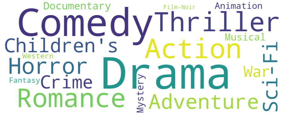

As you can see, the most frequent genres are Drama, Comedy and Action. We then have some other genres that are way less frequent such as Western, Fantasy or Sci-Fi. As I previously pointed out, the latter are those that we want to give the most importance to when recommending. But, why is that?

如您所见，最常见的类型是戏剧，喜剧和动作。然后，我们还有一些其他类型的频率较低的类型，例如西方，幻想或科幻。正如我之前指出的那样，后者是我们在推荐时最重视的内容。但是，为什么呢？

As an example let’s consider a user who wants to find a movie similar to “The Good, the Bad and the Ugly”, which is a mixture of Western, Action and Adventure. Which genre do you think will be more relevant in terms of recommending a movie to this user? Presumably Western, since there will be many Action or Adventure movies, which are not Western, which could lead to recommending many none Western movies.

作为示例，考虑一个想要查找类似于“ 善，恶，丑 ”的电影的用户，该电影是西方，动作和冒险的混合体。您认为哪种类型的电影与向该用户推荐电影更相关？大概是西方电影，因为将会有很多动作或冒险电影，而不是西方电影，这可能会导致推荐许多西方电影。

建立基于内容的推荐器 (Building a content based recommender)

For this post, we will be building quite a simple recommender, based on the movie genres. A fairly common approach for this problem is to use a tf-idf vectorizer.

对于本文，我们将根据电影流派建立一个非常简单的推荐器。解决此问题的一种相当普遍的方法是使用tf-idf矢量化器。

While this approach is more commonly used on a text corpus, it possesses some interesting properties that will be useful in order to obtain a vector representation of the data. The expression is defined as follows:

尽管这种方法更常用于文本语料库，但它具有一些有趣的属性，这些属性对于获取数据的矢量表示很有用。表达式定义如下：

Here we have the product of the term frequency, i.e. the amount of times a given term (genre) occurs in a document (genres of a movie), times the right side term, which basically scales the term frequency depending on the amount of times a given term appears in all documents (movies).

在这里，我们得到术语频率的乘积，即给定术语(流派)在文档(电影的流派)中出现的次数，乘以右侧术语的次数，这基本上取决于术语的出现次数给定的术语出现在所有文档(电影)中。

The fewer movies that contain a given genre (df_i), the higher the resulting weight. The logarithm is basically there to smooth the result of the division, i.e. avoids huge differences as a result of the right hand term.

包含给定类型( df_i)的电影越少，所得的权重就越高。对数基本上位于此处以使除法结果平滑，即避免因右手项而产生巨大差异。

So why is this useful in our case?

那么为什么这对我们来说有用呢？

As already mentioned, tf-idf will help capture the important genres of each movie by giving a higher weight to the less frequent genres, which we wouldn’t get with say, a CountVectorizer .

如前所述，tf-idf可以通过赋予较不频繁的流派更高的权重来帮助捕获每部电影的重要流派，而CountVectorizer 。

tf-idf (tf-idf)

To obtain the tf-idf vectors I’ll be using sklearn’s TfidfVectorizer . However, we have to take into account some aspects particular to this problem. The usual setup when dealing with text data, is to set a word analyser and perhaps an ngram_range , which will also include the n-grams within the specified range. An example would be:

为了获得tf-idf向量，我将使用sklearn的TfidfVectorizer 。但是，我们必须考虑到特定于此问题的某些方面。处理文本数据时，通常的设置是设置一个word分析器，也许还要设置一个ngram_range ，它还将包括指定范围内的n-gram。一个例子是：

from sklearn.feature_extraction.text import TfidfVectorizers = "Animation Children's Comedy"
tf_wrong = TfidfVectorizer(analyzer='word', ngram_range=(1,2))
tf_wrong.fit([s])
tf_wrong.get_feature_names()
# ['animation', 'animation children', 'children', 'children comedy', 'comedy']

However, that doesn’t really make sense in this case, since the order of the genres is not relevant, we want to account for the combinations of genres for a given movie, regardless of the order. So for the example above, we’d want:

但是，在这种情况下，这实际上没有任何意义，因为流派的顺序无关紧要，因此我们要考虑给定电影的流派组合，而与顺序无关。因此，对于上面的示例，我们想要：

from itertools import combinations
[c for i in range(1,4) for c in combinations(s.split(), r=i)]
[('Animation',),  ("Children's",),  ('Comedy',),  ('Animation', "Children's"),  ('Animation', 'Comedy'),  ("Children's", 'Comedy'),  ('Animation', "Children's", 'Comedy')]

Here we’re finding the sets of combinations of genres up to k (4 here), or in mathematical terms, the superset. Including the n>1 combinations of genres, will mean that the tf-idf vectorizer will also take into account how frequent these combinations are among all movies, assigning a higher score to those that appear the least.

在这里，我们找到了最大为k (此处为4)的类型组合的集合，或者用数学术语来说是superset 。包括n>1个流派组合，这意味着tf-idf矢量化器还将考虑这些组合在所有电影中的出现频率，并为出现最少的电影分配较高的分数。

We can apply the above logic using the analyser parameter, which we can use to obtain the sequence of features from the raw input using a callable:

我们可以使用analyser参数来应用以上逻辑，我们可以使用该参数通过可调用的方法从原始输入中获取特征序列：

tf = TfidfVectorizer(analyzer=lambda s: (c for i in range(1,4)
                     for c in combinations(s.split('|'), r=i)))
tfidf_matrix = tf.fit_transform(movies['genres'])
tfidf_matrix.shape
# (3883, 353)

This will result in the following tf-idf vectors (note that only a subset of the columns and rows is sampled):

这将导致以下tf-idf向量(请注意，仅对列和行的一部分进行了采样)：

pd.DataFrame(tfidf_matrix.todense(), columns=tf.get_feature_names(),   index=movies.title).sample(5, axis=1).sample(10, axis=0)

向量之间的相似性 (Similarity between vectors)

The next step will be to find similar tf-idf vectors (movies). Recall that we’ve encoded each movie’s genre into a tf-idf representation, now we want to define a proximity measure. A commonly used measure is the cosine similarity.

下一步将是寻找相似的tf-idf向量(电影)。回想一下，我们已经将每部电影的流派编码为tf-idf表示形式，现在我们要定义一个接近度度量。 常用的度量是余弦相似度。

This similarity measure owns its name to the fact that it equals to the cosine of the angle between the two vectors being compared. The lower the angle between two vectors, the higher the cosine will be, hence yielding a higher similarity factor. It is expressed as follows:

这种相似性度量的名称是它等于要比较的两个向量之间的角度的余弦。两个向量之间的角度越小，余弦将越高，因此产生更高的相似因子。表示如下：

Where, since the inner product can be expressed as the product of the magnitudes times the cosine of the angle between the two vectors, it becomes clear that the above can be expressed as the cosine:

其中，由于内积可以表示为大小乘以两个向量之间的角度的余弦的乘积，因此很显然，上述可以表示为余弦：

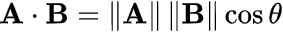
So the measure is obtained by taking the inner product between both vectors, and normalising by their respective magnitudes, resulting in the cosine between both vectors.

因此，通过获取两个向量之间的内积，并通过各自的幅度进行归一化，得出余弦值 两个向量之间。

To compute the cosine similarities between all tf-idf vectors, we can again use scikit-learn. sklearn.metrics.pairwise contains many pairwise distance metrics, among them cosine_similarity , which will compute the cosine similarities between all the input rows, in this case tf-idf vectors:

为了计算所有tf-idf向量之间的余弦相似度，我们可以再次使用scikit-learn。 sklearn.metrics.pairwise包含许多成对距离度量，其中cosine_similarity ，它将计算所有输入行之间的余弦相似度，在这种情况下为tf-idf向量：

from sklearn.metrics.pairwise import cosine_similarity
cosine_sim = cosine_similarity(tfidf_matrix)

Now we have to define some logic to find the highest weights or tf-idf scores for a given movie. For that I’ve defined the following function, which takes as input a given movie i, the similarity matrix M, the items dataframe and returns up to k recommendations:

现在，我们必须定义一些逻辑以找到给定电影的最高权重或tf-idf分数。为此，我定义了以下函数，该函数将给定电影i ，相似度矩阵M ，项目数据帧作为输入，并最多返回k建议：

def genre_recommendations(i, M, items, k=10):
    """
    Recommends movies based on a similarity dataframe

    Parameters
    ----------
    i : str
        Movie title (index of the similarity dataframe)
    M : pd.DataFrame
        Similarity dataframe, symmetric, with movies as indices and columns
    items : pd.DataFrame
        Contains both the title and some other features used to define similarity
    k : int
        Amount of recommendations to return

    """
    ix = M.loc[:,i].to_numpy().argpartition(range(-1,-k,-1))
    closest = M.columns[ix[-1:-(k+2):-1]]
    closest = closest.drop(i, errors='ignore')
    return pd.DataFrame(closest).merge(items).head(k)

By usingargpartition we take the k highest values in M(similarity matrix) on a given index (movie) i . We then index on the columns in M , and further slice to get from highest weights to lowest (excluding the the highest, which will be the same item, bare in mind that the matrix is symmetric, hence the 2s in the second line).

通过使用argpartition我们在给定索引(电影) i上获得M (相似性矩阵)中的k argpartition 。然后，我们在M的列上建立索引，并进一步切分以从最高权重到最低权重(不包括最高权重，该最高权重将是同一项目，请记住矩阵是对称的，因此第二行为2s )。

测试推荐器 (Testing the recommender)

Let’s test the recommender with a few examples. Since the movies dataset contains movies of up to 2000, we will have to be using some all time classics.

让我们通过一些示例测试推荐器。由于movies数据集中包含多达2000部电影，因此我们将不得不使用某些经典影片。

How about '2001: A Space Odyssey'?

那'2001: A Space Odyssey'怎么样？

movies[movies.title.eq('2001: A Space Odyssey (1968)')]
    movie_id                              title              genres
912      924       2001: A Space Odyssey (1968)  Drama|Mystery|Sci-Fi|Thriller

We can see that its genres are Drama|Mystery|Sci-Fi|Thriller . Let’s see what recommendations we get! :)

我们可以看到它的类型是Drama|Mystery|Sci-Fi|Thriller 。让我们看看我们得到什么建议！ :)

genre_recommendations('2001: A Space Odyssey (1968)', cosine_sim_df, movies[['title', 'genres']])

As expected, the most similar movies are those which share the most genres. Interestingly, we see that most of them are Sci-Fi movies. Note that this is likely to be influenced by the fact that Sci-Fi will mostly have the higher score among the genres that appear above, since it is the least frequent and hence has a higher weight.

不出所料，最相似的电影是类型最多的电影。有趣的是，我们看到其中大多数是Sci-Fi电影。请注意，这很可能受到以下事实的影响： Sci-Fi小说在上面出现的流派中得分最高，因为它的出现频率最低，因此权重更高。

Let’s try with Contact, of my fave Sci-Fi movies:

让我们尝试一下我最喜欢的科幻电影中的Contact ：

movies[movies.title.eq(‘Contact (1997)’)]
      movie_id           title        genres
1543      1584  Contact (1997)  Drama|Sci-Fi

In this case we’d get:

在这种情况下，我们将获得：

genre_recommendations('Contact (1997)', cosine_sim_df, movies[['title', 'genres']])

There seem to be many movies that share the same genres, hence we get all Drama|Sci-fi movies recommended.

似乎有很多电影具有相同的流派，因此我们推荐了所有Drama|Sci-fi电影。

Let’s try now with an animation movie like 'The Jungle Book':

现在，让我们尝试制作一部动画电影，例如'The Jungle Book' ：

movies[movies.title.eq('Jungle Book, The (1967)')]
      movie_id                    title                             
2009      2078  Jungle Book, The (1967) 
                             genres
Animation|Children's|Comedy|Musical

We get the following recommendations:

我们得到以下建议：

genre_recommendations('Jungle Book, The (1967)', cosine_sim_df, movies[['title', 'genres']])

There appear to be two movies that share the exact same combination of genres, and similarly with the rest but without the Comedy genre.

似乎有两部电影具有完全相同的流派组合，其余的相似，但没有Comedy流派。

Or let’s try with a last one, 'Saving private Ryan' :

或者让我们尝试最后一个'Saving private Ryan' ：

print(movies[movies.title.eq('Saving Private Ryan (1998)')])
      movie_id                       title            genres
1959      2028  Saving Private Ryan (1998)  Action|Drama|Wargenre_recommendations('Saving Private Ryan (1998)', cosine_sim_df, movies)

总结 (Concluding)

Overall, we’ve seen that quite a naive content based recommender can provide fairly good results.

总体而言，我们已经看到，基于幼稚的基于内容的推荐器可以提供相当好的结果。

A clear advantage of content based recommenders is that they don’t suffer from the cold-start problem, since we only need basic information on a user (in this case a single movie) to provide similar recommendations based on the items. Another interesting advantage is that we are able to recommend to users with unique tastes, which can be a lot more challenging with collaborative filtering methods.

基于内容的推荐器的明显优势在于它们不会遭受冷启动问题的困扰，因为我们只需要有关用户的基本信息(在本例中为单个电影)就可以根据项目提供类似的推荐。另一个有趣的优点是我们能够向用户推荐具有独特口味的产品，而使用协作过滤方法则可能更具挑战性。

An important drawback however is that it tends to recommend the same type of items to the user. In order to be able to recommend a different type of item, the user would have to have rated or have shown interest in the new type of item. This is a problem that Collaborative Filtering methods don’t have, since the match here is done between neighbouring users with similar tastes, but different items rated.

然而，一个重要的缺点是它倾向于向用户推荐相同类型的物品。为了能够推荐不同类型的项目，用户将必须对新类型的项目进行评级或表现出兴趣。这是协作过滤方法所没有的问题，因为此处的匹配是在口味相似但评分不同的相邻用户之间完成的。

Thanks for reading!

谢谢阅读！