svm内核它们实际做什么

最新推荐文章于 2023-03-29 21:40:35 发布

weixin_26704853

最新推荐文章于 2023-03-29 21:40:35 发布

阅读量507

点赞数

文章标签： java linux

原文链接：https://towardsdatascience.com/svm-kernels-what-do-they-actually-do-56ce36f4f7b8

版权

You may have heard about the so-called kernel trick, a maneuver that allows support vector machines, or SVMs, to work well with non-linear data. The idea is to map the data into a high-dimensional space in which it becomes linear and then apply a simple, linear SVM. Sounds sophisticated and to some extent it is. However, while it might be hard to understand how the kernels work, it is pretty easy to grasp what they are trying to achieve. Read on to see it for yourself!

您可能已经听说过所谓的内核技巧，该技巧使支持向量机或SVM可以很好地处理非线性数据。想法是将数据映射到一个高维空间，在该空间中它变为线性，然后应用简单的线性SVM。听起来很复杂，在某种程度上说确实如此。但是，尽管可能很难理解内核的工作方式，但是很容易掌握内核要实现的目标。继续阅读以亲自体验！

当数据是线性可分离的时：线性SVM (When data are linearly separable: a linear SVM)

First things first: how does the vanilla SVM work? We can use SVMs for both classification and regression tasks, but in this article, we’ll focus on the former. Let’s first consider data with two classes that are linearly separable. We will create two separate blobs of points and fit a linear SVM to them using scikit-learn. Note that we normalize the data before fitting the model since SVMs are sensitive to features’ scales.

首先，第一件事：香草SVM如何工作？我们可以将SVM用于分类和回归任务，但是在本文中，我们将重点关注前者。我们首先考虑具有线性可分离的两个类别的数据。我们将创建两个单独的点斑点，并使用scikit-learn将线性SVM拟合到它们。请注意，由于SVM对要素比例敏感，因此我们在拟合模型之前先对数据进行归一化。

X, y = make_blobs(n_samples=100, centers=2, n_features=2, random_state=42)
pipe = make_pipeline(StandardScaler(), LinearSVC(C=1, loss="hinge"))
pipe.fit(X, y)


plot_svm(pipe, X)

The customplot_svm() function, the output of which you can see below, consists of quite some matplotlib code — you can check it out in this jupyter notebook if you’re curious.

自定义plot_svm()函数plot_svm()您可以在下面看到其输出plot_svm()包含一些matplotlib代码-您可以在此查看 jupyter笔记本(如果您很好奇)。

There are many lines that separate the two classes perfectly, infinitely many, to be exact. The line fitted by the SVM is special in that it is the middle line of a band marked with the dashed lines, and this band is the widest possible band that can be squeezed between the two classes. This way, the SVM decision line (marked as a solid black line) is as far from both classes as possible, ensuring the model will generalize well to new examples.

确切地说，有许多行将两个类完美地分开，无限多个。 SVM拟合的线是特殊的，因为它是用虚线标记的带的中间线，并且该带是可以在两类之间压缩的最大宽度的带。这样，SVM决策线(标为实心黑色线)尽可能远离两个类，从而确保模型可以很好地推广到新示例。

The observations on the border of the band circled in red are called support vectors since they support, or determine, the location of the band. Should we add some observations outside the band, it would not change position.

用红色圈出的带边界上的观察值称为支持向量，因为它们支持或确定带的位置。如果我们在频带之外添加一些观察，则不会改变位置。

As a side note: this is an example of hard-margin classification, which means no observations are allowed into the band. Alternatively, we could do a soft-margin classification: allow some observation into the band, but not too many, making the band even wider at the same time. That would be more robust against outliers and can be controlled by the parameter C in LinearSVC(): we have set it to 1, but decreasing it to 0.1, for instance, would result in a wider band, but with some observations inside it. Anyway, this is not that relevant to our story.

附带说明：这是硬边距分类的示例，这意味着不允许在波段中进行观察。或者，我们可以进行软边距分类：允许对频段进行一些观察，但不要太多，从而可以使频段同时变宽。这样可以更好地抵御离群值，并且可以通过LinearSVC()的参数C进行控制：我们将其设置为1，但是例如将其减小到0.1，则会得到较宽的频带，但其中会有一些观察结果。无论如何，这与我们的故事无关。

Most real-life data sets are not nice, linearly separable blobs. Let’s see how the linear SVM handles moon-shaped data.

大多数现实生活中的数据集都不是很好的线性可分离斑点。让我们看看线性SVM如何处理月亮形状的数据。

X, y = make_moons(n_samples=100, noise=0.1, random_state=42)
pipe = make_pipeline(StandardScaler(), LinearSVC(C=1, loss="hinge"))
pipe.fit(X, y)


plot_svm(pipe, X)

This doesn’t look good, does it? Let’s see what we can do about it.

这看起来不好，是吗？让我们看看我们能做些什么。

映射到更高的尺寸 (Mapping to higher dimensions)

Before we discuss the kernels and what they do, let’s first look at one powerful idea they make use of: in a high dimensional space, there is a bigger chance the data will become linearly separable.

在讨论内核及其作用之前，我们首先来看一下它们利用的一个有力想法：在高维空间中，数据变得线性可分离的可能性更大。

This is clearly illustrated by the following pair of plots. When we only have one feature, x1, we cannot separate the data with a single line. Adding another feature, x2, equal to x1 squared, makes it easy to separate the two classes.

下面的一对图清楚地说明了这一点。当我们只有一个特征x1时 ，我们不能用一行来分隔数据。添加另一个等于x1平方的特征x2，可以很容易地将两个类分开。

反正什么是内核？ (What is a kernel anyway?)

So, what is the kernel trick about? Kernels are simply a smart way of adding more features to the data in the hope of making it linearly separable. Smart, because instead of actually adding them, which would make the model slow, they make use of some magical mathematical properties (which are out of scope of this article) that allow us to obtain exactly the same results as if we had actually added these features, without slowing the model down.

那么，内核技巧是什么呢？内核只是向数据添加更多功能以使其线性分离的一种聪明方法。聪明，因为它们没有实际添加它们(这会使模型变慢)，而是利用了一些神奇的数学属性(超出了本文的范围)，这些属性使我们可以获得与实际添加这些结果完全相同的结果功能 ，而不会降低模型速度。

Two popular kernels are the polynomial kernel and the Gaussian Radial Basis Function, or RBF, kernel. They differ in the types of features that they (pretend to) add. Let’s look at what they do!

两种流行的内核是多项式内核和高斯径向基函数或RBF内核 。它们在(假装)添加的功能类型上有所不同。让我们看看他们在做什么！

具有多项式核的多项式特征 (Polynomial features with polynomial kernel)

One way to create more features is to use their polynomial combinations up to a certain degree. For instance, with two features A and B, a polynomial of degree 2 would produce 6 features: 1 (any feature to power 0), A, B, A², B², and AB. We can easily add these features manually with scikit-learn’s PolynomialFeatures():

创建更多特征的一种方法是在一定程度上使用其多项式组合。例如，对于两个特征A和B，一个2阶多项式将产生6个特征：1(任何幂为0的特征)，A，B，A²，B²和AB。我们可以使用scikit-learn的PolynomialFeatures()轻松地手动添加这些功能：

X, y = make_moons(n_samples=100, noise=0.1, random_state=42)
pipe = make_pipeline(StandardScaler(), 
                     PolynomialFeatures(degree=3), 
                     LinearSVC(C=5))
pipe.fit(X, y)
plot_svm(pipe, X)

or we can simply use a polynomial kernel:

或者我们可以简单地使用多项式内核：

X, y = make_moons(n_samples=100, noise=0.1, random_state=42)
pipe = make_pipeline(StandardScaler(), SVC(kernel="poly", degree=3, C=5, coef0=1))
pipe.fit(X, y)


plot_svm(pipe, X)

You can verify yourself that both implementations yield roughly identical plots, somewhat like this:

您可以验证自己，两个实现产生的图形大致相同，如下所示：

The advantage of using the kernelized version is that you can specify the degree to be large, thus increasing the chance that data will become linearly separable in this high-dimensional space, without slowing the model down.

使用内核版本的优势在于，您可以指定较大的程度，从而增加数据在此高维空间中线性分离的机会，而不会降低模型的速度。

For our moon-data example, it is clear from the scatter plot that a polynomial of degree 3 would be enough. For more complex datasets, however, you might need to use a higher degree. This is when the power of the kernel trick is unleashed.

对于我们的卫星数据示例，从散点图中可以明显看出，阶数为3的多项式就足够了。但是，对于更复杂的数据集，您可能需要使用更高的度数。这是释放内核技巧的力量的时候。

与高斯RBF内核的相似性 (Similarity features with Gaussian RBF kernel)

Another method to add more features to the data is to use the so-called similarity features. A similarity feature measures how far a value of an existing feature is from a landmark. Let’s make it practical: we have a data set with a single feature, x1. We want to create two similarity features, so we select two landmarks, i.e. reference values from our single feature. Let’s take -1 and 1, for instance. Then, for each value of x1, we calculate how far it is from the first landmark (read on to see how to define ‘far’). This is our new similarity feature, x2. Then we do the same, comparing values of x1 to the second landmark to obtain x3. Now we don’t even need the original feature x1! The two new similarity features make our data easily separable.

向数据添加更多特征的另一种方法是使用所谓的相似性特征。相似特征用于度量现有特征的值与地标的距离。让我们付诸实践：我们有一个具有单个功能x1的数据集。我们要创建两个相似性特征，因此我们选择两个界标，即从单个特征中选择参考值。让我们以-1和1为例。然后，对于x1的每个值，我们计算距第一个界标的距离(请继续阅读以了解如何定义“远”)。这是我们的新相似性功能x2 。然后，我们将x1的值与第二个界标进行比较，以获得x3 。现在，我们甚至不需要原始功能x1 ！这两个新的相似性功能使我们的数据易于分离。

So, how do we calculate the distance of each observation from the landmark? A popular choice is to use the Gaussian Radial Basis Function, or RBF. It is defined as:

那么，我们如何计算每个观测点到地标的距离？流行的选择是使用高斯径向基函数或RBF。它定义为：

where x is our original feature and γ is a parameter, which I set to be 0.3.

其中x是我们的原始特征，而γ是参数，我将其设置为0.3。

For example, the first observation scores -3 on our only original feature. We computed x2 as exp(-0.3 * (-3-(-1))²)≈0.30, and x3 as exp(-0.3 * (-3-(1))²)≈0.01. That’s the bottom-most dot on the right-hand-side plot.

例如，第一个观察结果在我们唯一的原始特征上得分为-3。我们将x2计算为exp(-0.3 *(-3-(-1))²)≈0.30，将x3计算为exp(-0.3 *(-3-(1))²)≈0.01。那是右侧图的最底下的点。

In the above example, we have luckily chosen two landmarks that happened to work well. In practice, one might need a lot of landmarks, which translates to many new similarity features. That would slow the SVM down a lot — unless we resort to the kernel trick! Analogous to the polynomial kernel, the RBF kernel allows us to obtain exactly the same results as though we had added a landmark at each value of the original feature without the need to actually do it. Let’s try it out at our moon-shaped data.

在上面的示例中，我们幸运地选择了两个碰巧运行良好的地标。在实践中，可能需要很多地标，这会转化为许多新的相似性特征。这将大大降低SVM的速度-除非我们诉诸内核技巧！与多项式内核类似，RBF内核使我们可以获得完全相同的结果，就像我们在原始特征的每个值处添加了界标一样，而无需实际执行。让我们在月球形数据上尝试一下。

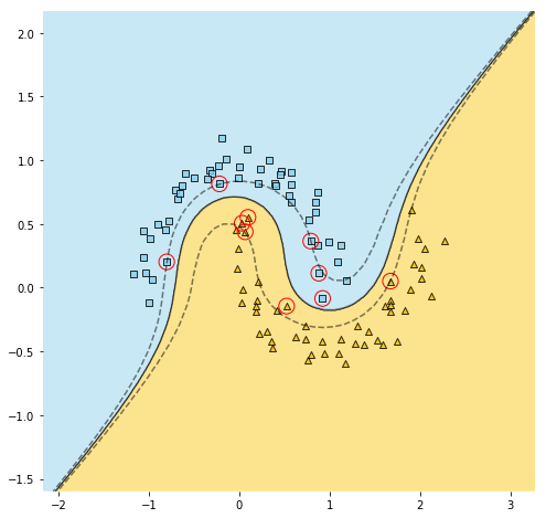
X, y = make_moons(n_samples=100, noise=0.1, random_state=42)
pipe = make_pipeline(StandardScaler(), SVC(kernel="rbf", gamma=0.3, C=5))
pipe.fit(X, y)


plot_svm(pipe, X)

The decision boundary looks pretty decent, but you might have noticed some misclassified examples. We can fix it by tuning the γ parameter. It acts as a regularizer — the smaller it is, the smoother the decision boundary, which prevents overfitting. In this case, however, we seem to actually be underfitting, so let’s increase γ to 0.5.

决策边界看起来相当不错，但是您可能已经注意到一些错误分类的示例。我们可以通过调整γ参数来修复它。它充当正则化器-越小，决策边界越平滑，从而防止过度拟合。但是，在这种情况下，我们似乎实际上是拟合不足的，因此让我们将γ增加到0.5。

Now all examples have been classifier correctly!

现在，所有示例均已正确分类！

摘要 (Summary)

Support Vector Machines perform classification by finding linear decision boundaries that are as far away from the data as possible. They work great with linearly separable data but fail miserably otherwise.
支持向量机通过查找距离数据尽可能远的线性决策边界来执行分类。它们可以很好地处理线性可分离的数据，但否则会失败。
To make non-linear data linearly separable (and thus convenient for SVMs) we can add more features to the data since in a higher-dimensional space the probability of the data being linearly separable increases.
为了使非线性数据线性可分离(因此对于SVM方便)，我们可以为数据添加更多功能，因为在高维空间中，数据线性可分离的可能性增加。
Two popular types of new features to add are polynomial combinations of existing features (polynomial features) and observation-wise distances from landmarks, i.e. some reference values (similarity features).
新增的两种流行类型的新特征是现有特征的多项式组合(多项式特征)和到地标的观察距离，即一些参考值(相似性特征)。
Actually adding them might slow the model down to the extent of making it useless.
实际上添加它们可能会使模型减慢到使其无法使用的程度。
The kernel trick is a smart maneuver that takes advantage of some mathematical properties in order to deliver the same results as though we have added additional features without actually adding them.
内核技巧是一种聪明的操作，它利用某些数学属性来提供相同的结果，就像我们添加了其他功能而没有实际添加它们一样。
The polynomial and RBF kernels (pretend to) add the polynomial and similarity features, respectively.
多项式和RBF内核(假装为)分别添加了多项式和相似性特征。

资料来源 (Sources)

Geron A., 2019, 2nd edition, Hands-On Machine Learning with Scikit-Learn and TensorFlow: Concepts, Tools, and Techniques to Build Intelligent Systems
Geron A.，2019年，第二版，使用Scikit-Learn和TensorFlow进行动手机器学习：构建智能系统的概念，工具和技术

Thanks for reading! I hope you have learned something useful that will boost your projects 🚀

谢谢阅读！我希望您学到了一些有用的东西，可以促进您的项目projects

You can find the data and the code for this post (including plotting) here. If you liked this post, try one of my other articles. Can’t choose? Pick one of these:

您可以在此处找到此帖子的数据和代码(包括绘图) 。如果您喜欢这篇文章，请尝试我的其他文章之一。无法选择？选择以下之一：