如何训练神经网络进行图像分类第1部分

Image classification is a hot topic in data science with the past few years seeing huge improvements in many areas. It has a lot of applications everywhere including SEO. But how is this done?

图像分类是数据科学中的一个热门话题，在过去的几年中，图像分类在许多领域都取得了巨大的进步。 它到处都有很多应用程序，包括SEO。 但是，这是怎么做的呢？

A deep neural network is a network of artificial neurons organised into layers (via software). With each layer connected to the next and each connection having a weight that helps determine how much the artificial neuron fires. This firing helps determine how strong the connections are between layers, and in general neurons that fire together have stronger connections. Just like with biological neurons.

深神经网络是组织成的人工神经元网络层 (通过软件)。 每个层都连接到下一层，并且每个连接的权重都有助于确定人造神经元的发射量。 这种发射有助于确定各层之间的连接强度，通常，一起发射的神经元具有更强的连接。 就像生物神经元一样。

How strong these connections are is determined by how the network is trained on the data you put into it. These networks are trained via a process called backpropagation which works to feed data into the network and then measures the network’s performance. This error is measured using a loss function.

这些连接的牢固程度取决于如何根据输入的数据对网络进行培训 。 这些网络是通过称为反向传播的过程进行训练的，该过程将数据馈入网络，然后测量网络的性能。 使用损耗函数测量该误差。

Backpropagation works by using gradient descent to measure the rate-of-change of the loss function with respect to the weighting of each connection, and the gradient descent step is used to make sure the error rate for each connection is reduced as close to zero as possible. The network should eventually converge on a solution where the overall error is minimised.

反向传播通过使用梯度下降来测量损耗函数相对于每个连接权重的变化率来进行工作，并且使用梯度下降步骤来确保将每个连接的错误率降低到接近零。可能。 网络最终应收敛于最小化总体误差的解决方案。

The rate at which the network learns is called the learning rate and this is another hyperparameter that can be tuned when training neural networks. If the learning rate is too small, the network can take too long to converge on a solution, and conversely, if the learning rate is too large then the network will ‘bounce around’ and never really converge on an optimum solution.

网络学习的速率称为学习速率，这是训练神经网络时可以调整的另一个超参数。 如果学习率太小，则网络可能花费太长时间才能收敛于解决方案，反之，如果学习率太高，则网络将“反弹”并且永远不会真正收敛于最佳解决方案。

There are different types of layers in neural networks, and each one transforms data differently. The most basic type is a dense layer, which is where all neurons are connected. Other types include convolutional layers which are primarily used for image processing tasks and recurrent layers which are used to process time-series data. There are others, but these are the most common types.

神经网络中有不同类型的层，并且每个层对数据的转换都不同。 最基本的类型是密集层，这是所有神经元连接的地方。 其他类型包括主要用于图像处理任务的卷积层和用于处理时间序列数据的循环层。 还有其他类型，但是这些是最常见的类型。

In this article, I will be focusing on how to implement a simple image classifier using a series of dense layers in Python using Keras as part of Tensorflow. As mentioned above, convolutional neural networks usually work better for image classification tasks and I will talk about these in part 2 of this series. As my primary area of interest is Search Engine Optimisation, I will tie all of this together in part 3 for how neural networks are used in search.

在这篇文章中，我将重点放在如何实现使用一系列使用Python中的致密层的一个简单的图像分类Keras作为一部分Tensorflow 。 如上所述，卷积神经网络通常可以更好地用于图像分类任务，我将在本系列的第2部分中讨论这些问题。 由于我的主要兴趣是搜索引擎优化，因此我将在第3部分中将所有这些联系在一起，以了解如何在搜索中使用神经网络。

Neural networks are fascinating, and if you have an interest in this topic, I would encourage you to check out this excellent playlist on YouTube on a channel called Deep Lizard. They have excellent and accessible content on neural networks and deep learning.

神经网络令人着迷，如果您对此主题感兴趣，我鼓励您在YouTube上名为Deep Lizard的频道上查看这个出色的播放列表 。 他们在神经网络和深度学习方面拥有出色且易于访问的内容。

If you are more interested in the implementation using Python with Keras, I would encourage you to look at Hands-on Machine Learning with Scikit-Learn, Keras and Tensorflow by Aurelion Geron. It is an excellent book, written by a former Googler and reviewed by the author of Keras. I highly recommend it.

如果您对将Python与Keras结合使用的实现更感兴趣，我鼓励您看看Aurelion Geron的Scikit-Learn，Keras和Tensorflow的动手机器学习 。 这是一本非常棒的书，由前Google员工撰写，并由Keras的作者撰写。 我强烈推荐它。

Keras和TensorFlow入门 (Getting started with Keras and TensorFlow)

Keras is a high-level deep learning API in Python that allows you to easily create and train deep learning models. It was launched in 2016 and has gained traction within the data science community due to its ease-of-use as its syntax is designed to be very similar to Scikit-Learn.

Keras是Python中的高级深度学习API，可让您轻松创建和训练深度学习模型。 它于2016年推出，由于其易用性而在数据科学界引起了广泛关注，因为其语法设计与Scikit-Learn非常相似。

TensorFlow is a library created by the Google Brain team for machine learning tasks and has often competed with PyTorch (created by Facebook) for market share, but has not been able to do as well as its documentation wasn’t as accessible. To remedy this, Google released TensorFlow 2 which contained many improvements particularly around cross-compatibility with models, GPU support and graphing utilities.

TensorFlow是由Google Brain团队创建的用于机器学习任务的库，经常与PyTorch (由Facebook创建)争夺市场份额，但由于无法提供文档而无法做到。 为了解决这个问题，Google发布了TensorFlow 2，其中包含许多改进，特别是在与模型，GPU支持和图形实用程序的交叉兼容性方面。

With the release of TensorFlow 2, Keras is now merged into Tensorflow and the standalone version is no longer maintained. If you want to install Keras and TensorFlow then it is straightforward. Just go to your Python environment (I recommend using a virtual environment/package manager like pipenv) and use whichever Python package manager you like:

随着TensorFlow 2的发布，Keras现在已合并到Tensorflow中，并且不再维护独立版本。 如果您要安装Keras和TensorFlow，那么它很简单。 只需转到您的Python环境(我建议使用虚拟环境/程序包管理器，如pipenv )，然后使用您喜欢的任何Python程序包管理器：

python -m pip install TensorFlow

Be sure to use a 64-bit version of Python for this to work. To get GPU support on Windows is a bit of a faff, but this YouTube video will show you how to get it done. However, you probably won’t need it for this tutorial. You could look at Google Colab as that has GPUs available with no setup.

确保使用64位版本的Python才能正常工作。 在Windows上获得GPU支持有点麻烦，但是此YouTube 视频将向您展示如何完成它。 但是，本教程可能不需要它。 您可以查看Google Colab，因为它具有没有设置的可用GPU。

You can check the installation in a Jupyter notebook with the following:

您可以使用以下命令在Jupyter笔记本中检查安装：

import TensorFlow as tf
from tensorflow import keras
print(tf.__version__)
print(keras.__version__)

If this has all worked, then at the time of writing you should see something like:

如果一切都成功了，那么在撰写本文时，您应该会看到类似以下内容的内容：

2.3.0
2.4.0

When you’ve got Keras and TensorFlow working, you should be good to go on building an image classifier with a neural network.

当Keras和TensorFlow工作时，您应该继续使用神经网络构建图像分类器。

导入数据集 (Importing the data set)

For most simple image classification tasks, it is popular to use the MNIST data set, which consists of 60,000 photos of handwritten numbers. However, for this task, we are going to use the MNIST Fashion dataset, which consists of 60,000 28 x 28 grayscale images of Zalando article fashion images, all classified across 10 different classes. The reason for this is that image classifiers tend to find this more challenging.

对于大多数简单的图像分类任务，通常使用MNIST数据集 ，该数据集包含60,000张手写数字的照片。 但是，对于此任务，我们将使用MNIST Fashion数据集 ，该数据集由Zalando文章时尚图像的60,000张28 x 28灰度图像组成，所有图像均分为10个不同的类。 这样做的原因是图像分类器趋向于更具挑战性。

Keras has utility functions to help import this dataset, so it is fairly straightforward to use (similar to Sklearn). Work in a Jupyter notebook, and begin by making sure we have all the imports we need:

Keras具有实用程序功能来帮助导入该数据集，因此使用起来相当简单(类似于Sklearn)。 在Jupyter笔记本中工作，并首先确保我们拥有所需的所有进口物品：

import tensorflow as tf
from tensorflow import keras
import numpy as np
import pandas as pd
import matplotlib.pyplot as plt

We will be working with NumPy arrays and plotting this with Matplotlib, so you will need to ensure these are accessible within your environment. Once this is done, you can import the dataset:

我们将使用NumPy数组，并使用Matplotlib进行绘制，因此您需要确保可以在您的环境中访问它们。 完成此操作后，您可以导入数据集：

fashion_mnist = keras.datasets.fashion_mnist
(X_train_full, y_train_full), (X_test, y_test) = fashion_mnist.load_data()

The dataset is split between a training and a test set automatically (60,000 images in training, 10,000 images in test). The x-axis data are the images and the y-axis data are the labels. To make this more useful for working with, it is also a good idea to create a validation data set so we can ensure the model isn’t overfitting:

数据集自动在训练集和测试集之间划分(训练中60,000张图像，测试中10,000张图像)。 x轴数据是图像，y轴数据是标签。 为了使它更有用，创建验证数据集也是一个好主意，这样我们可以确保模型不会过拟合：

X_valid, X_train = X_train_full[:5000] X_train_full[5000:]
y_valid, y_train = y_train_full[:5000], y_train_full[5000:]

The y-axis data is just a series of numbers associated with each class label, therefore we need to define the class labels manually:

y轴数据只是与每个类别标签相关的一系列数字，因此我们需要手动定义类别标签：

class_names = [ “T-shirt/top” , “Trouser” , “Pullover” , “Dress” , “Coat” , “Sandal” , “Shirt” , “Sneaker” , “Bag” , “Ankle boot” ]

To get an idea of what the dataset actually represents we can use a simple loop and Matplotlib:

为了了解数据集实际代表什么，我们可以使用一个简单的循环和Matplotlib：

plt.figure(figsize=(10,10))
for i in range(25):
    plt.subplot(5,5,i+1)
    plt.xticks([])
    plt.yticks([])
    plt.grid(False)
    plt.imshow(X_train_full[i], cmap=plt.cm.binary)
    plt.xlabel(class_names[y_train_full[i]])
plt.show()

From this, you will see something like this:

由此，您将看到类似以下内容：

First 25 entries from the Fashion MNIST dataset

Fashion MNIST数据集中的前25个条目

As you can, while there are only 10 classes (similar to the MNIST dataset), the images are different for each class, which is why it is a more challenging dataset to work with.

如您所愿，虽然只有10个类别(类似于MNIST数据集)，但是每个类别的图像都不相同，这就是使用它更具挑战性的数据集的原因。

标准化数据集 (Normalizing the dataset)

The first step to working with neural networks is to normalize the dataset, otherwise, it could take a lot longer for the network to converge on a solution.

使用神经网络的第一步是对数据集进行规范化，否则，网络收敛到解决方案可能会花费更长的时间。

The usual way of normalizing a dataset is to scale the features, and this is done by substacting the mean from each feature and dividing by the standard deviation. This will put the features on the same scale somewhere between 0 — 1.

标准化数据集的通常方法是缩放特征，这是通过将每个特征的均值除以标准差来完成的。 这会将要素以相同的比例置于0到1之间。

As we are working with 28 x 28 NumPy arrays representing each image and each pixel in the array has an intensity somewhere between 1 — 255, a simpler way of getting all of these images on a scale between 0–1 is to divide each array by 255.

当我们使用表示每个图像的28 x 28 NumPy数组，并且数组中的每个像素的强度介于1到255之间时，将所有这些图像缩放为0–1的简单方法是将每个数组除以255。

X_valid, X_train = X_train_full / 255., X_train_full / 255.
X_test = X_test / 255.

From there, we are good to go to build a dense layer neural network and train it on our data set.

从那里开始，我们很高兴去构建一个密集层神经网络，并在我们的数据集上对其进行训练。

建立神经网络图像分类器 (Building the neural network image classifier)

In order to build the model, we have to specify its structure using Keras’ syntax. As mentioned above, it is very similar to Scikit-Learn and so it should be recognisable if you are familiar with that package. The code for building the model is as follows:

为了构建模型，我们必须使用Keras的语法指定其结构。 如上所述，它与Scikit-Learn非常相似，因此如果您熟悉该软件包，则应该可以识别。 用于构建模型的代码如下：

model = keras.models.Sequential([keras.layers.Flatten(input_shape = [28, 28]),
keras.layers.Dense(300, activation = “relu” ),
keras.layers.Dense(100, activation = “relu” ),
keras.layers.Dense(100, activation = “relu” ),
keras.layers.Dense(100, activation = “relu” ),
keras.layers.Dense(10, activation = “softmax” )])

To explain this code:

解释此代码：

• The first line creates a Sequential model and this is the simplest type of data structure in Keras and is basically a sequence of connected layers in a network

  第一行创建一个顺序模型，这是Keras中最简单的数据结构类型，基本上是网络中一系列连接的层

• The first layer in the model is a flatten layer and is there for pre-processing of the data and it isn’t trainable itself. What this does is take each 28 x 28 NumPy array for each image and flattens it into a 1 x 784 array that the network can work with

  模型中的第一层是扁平层，用于数据的预处理，它本身不可训练。 这样做是为每个图像取每个28 x 28 NumPy数组并将其展平为网络可以使用的1 x 784数组

• Next, we add a Dense hidden layer with 300 neurons. It will use the ReLU activation function. Each Dense layer manages its own weight matrix, containing all the connection weights between the neurons and their inputs

  接下来，我们添加具有300个神经元的密集隐藏层。 它将使用ReLU激活功能。 每个密集层管理自己的权重矩阵，其中包含神经元及其输入之间的所有连接权重

• Next, we add another 3 Dense layers with 100 neurons each. There are diminishing returns to adding new layers and this is something we need to test as we build and optimise the network

  接下来，我们再添加3个Dense层，每个层有100个神经元。 添加新层的收益递减，这是我们在构建和优化网络时需要测试的东西

• Finally, we add a Dense layer with 10 neurons as there are 10 classes to predict and as they are all exclusive, we use the softmax activation function

  最后，我们添加了一个包含10个神经元的密集层，因为要预测10个类，并且它们都是排他性的，因此我们使用softmax激活函数

To get a full understanding of the model’s structure we can use:

为了全面了解模型的结构，我们可以使用：

model.summary()

And this will give us an output of the full structure of the network:

这将为我们提供网络完整结构的输出：

Model: “sequential_2” _________________________________________________________________ Layer (type) Output Shape Param # ================================================================= flatten_2 (Flatten) (None, 784) 0 _________________________________________________________________ dense_10 (Dense) (None, 300) 235500 _________________________________________________________________ dense_11 (Dense) (None, 100) 30100 _________________________________________________________________ dense_12 (Dense) (None, 100) 10100 _________________________________________________________________ dense_13 (Dense) (None, 100) 10100 _________________________________________________________________ dense_14 (Dense) (None, 10) 1010 ================================================================= Total params: 286,810 Trainable params: 286,810 Non-trainable params: 0 _________________________________________________________________

As can be seen this network has a total of 286,810 trainable parameters (consisting of weights between neurons and bias terms) and this gives the network a lot of flexibility, but it also means that it will be very easy for it to overfit so we need to becareful.

可以看出，该网络总共有286,810个可训练参数(由神经元和偏差项之间的权重组成)，这为网络提供了很大的灵活性，但是这也意味着它很容易过度拟合，因此我们需要要小心。

Before we can train the network we need to compile it, and this is done with the following code:

在训练网络之前，我们需要对其进行编译，这是通过以下代码完成的：

model.compile(loss = “sparse_categorical_crossentropy”,
optimizer = “sgd”,
metrics = [“accuracy”])

In this line we are specifying 3 things:

在这一行中，我们指定了三件事：

i) The loss function to use. In this case we are using sparse categorical cross entropy — this is because we have an index of exclusive (sparse) labels we are trying to predict against

i)损失函数。 在这种情况下，我们使用稀疏分类交叉熵 -这是因为我们有一个我们试图针对的排他(稀疏)标签索引

ii) The optimizer we are going to use to optimise the model against the loss function is stochastic gradient descent and this will ensure the model converges on an optimum solution i.e. Keras will use the backpropagation method described above

ⅱ)我们将用它来优化对损失函数模型中的优化是随机梯度下降 并确保模型收敛于最佳解，即Keras将使用上述反向传播方法

iii) Finally, we specify a metric that we are going to use in addition to loss to give us an idea of how well our model is working. In this case, we are using accuracy which gives an idea of how well our model is doing by giving a percentage of how many predictions match the actual class for the model we are training

iii)最后，我们指定除损失外将要使用的度量，以使我们了解模型的运行状况。 在这种情况下，我们使用准确性 通过给出多少预测与我们正在训练的模型的实际类别相匹配的百分比，可以了解模型的运行状况

训练网络 (Training the network)

Training the network is easy once it has been compiled. All you need to do is call the model’s fit method (like Sklearn) as follows:

编译网络后，对网络进行培训很容易。 您需要做的就是调用模型的fit方法(例如Sklearn)，如下所示：

history = model.fit(X_train,
                    y_train,
                    epochs = 10,
                    validation_data = (X_valid, y_valid))

We initially pass in the data that we want to train the network on, in this case, X_train are the images and y_train is an array containing the labels. We also specify the number of epochs we want to train the model with (an epoch being defined as how many times we want to pass the training data through the network for training purposes).

最初，我们传递要在其上训练网络的数据，在这种情况下， X_train是图像， y_train是包含标签的数组。 我们还指定了要用来训练模型的时期数(一个时期被定义为我们想要通过训练网络将训练数据传递多少次)。

Keras also lets us specify an optional validation_data argument where we pass in a validation data set. If we do this, then at the end of each epoch Keras will test the performance of the network on the validation data set. This is a good way of ensuring the model isn’t overfitting, however, it doesn’t feed into the training itself.

Keras还允许我们指定一个可选的validation_data参数，在该参数中传递验证数据集。 如果我们这样做，那么在每个纪元末，Keras将在验证数据集上测试网络的性能。 这是确保模型不过度拟合的好方法，但是，它不会影响训练本身。

As training proceeds, you will see something like this:

随着培训的进行，您将看到以下内容：

Epoch 1/10 1719/1719 [==============================] — 5s 3ms/step — loss: 0.7698 — accuracy: 0.7385 — val_loss: 0.5738 — val_accuracy: 0.7962 
Epoch 2/10 1719/1719 [==============================] — 5s 3ms/step — loss: 0.4830 — accuracy: 0.8283 — val_loss: 0.4570 — val_accuracy: 0.8404 
Epoch 3/10 1719/1719 [==============================] — 5s 3ms/step — loss: 0.4261 — accuracy: 0.8480 — val_loss: 0.4121 — val_accuracy: 0.8522 
Epoch 4/10 1719/1719 [==============================] — 5s 3ms/step — loss: 0.3932 — accuracy: 0.8582 — val_loss: 0.3951 — val_accuracy: 0.8566 
Epoch 5/10 1719/1719 [==============================] — 5s 3ms/step — loss: 0.3708 — accuracy: 0.8660 — val_loss: 0.3597 — val_accuracy: 0.8682 
Epoch 6/10 1719/1719 [==============================] — 5s 3ms/step — loss: 0.3518 — accuracy: 0.8728 — val_loss: 0.3397 — val_accuracy: 0.8756 
Epoch 7/10 1719/1719 [==============================] — 5s 3ms/step — loss: 0.3369 — accuracy: 0.8779 — val_loss: 0.3506 — val_accuracy: 0.8738 
Epoch 8/10 1719/1719 [==============================] — 5s 3ms/step — loss: 0.3243 — accuracy: 0.8814 — val_loss: 0.3343 — val_accuracy: 0.8774 
Epoch 9/10 1719/1719 [==============================] — 4s 3ms/step — loss: 0.3128 — accuracy: 0.8861 — val_loss: 0.3415 — val_accuracy: 0.8794 
Epoch 10/10 1719/1719 [==============================] — 4s 2ms/step — loss: 0.3019 — accuracy: 0.8888 — val_loss: 0.3265 — val_accuracy: 0.8822

This will continue for as long as the training is happening, there are accuracy and loss metrics for both the training and validation data sets. The value of the accuracy is a simple percentage measure of how many items the network got right. The value of loss is the cross entropy loss.

只要训练正在进行，这种情况就会持续下去，训练和验证数据集都有准确性和损失指标。 准确性的值是对网络中正确的项目数的简单百分比度量。 损失的价值就是交叉熵损失 。

Once the model is trained, it is possible to call its history method to get a dictionary of the loss and any other metrics needed at every stage of the training. We can put these in a Pandas DataFrame and plot them as follows:

训练模型后，可以调用其历史记录方法以获取损失的字典以及训练每个阶段所需的任何其他指标。 我们可以将它们放在Pandas DataFrame中，并按以下方式绘制它们：

pd.DataFrame(history.history).plot(figsize = (16, 10))
plt.grid(True)
plt.gca().set_ylim(0, 1)
plt.show()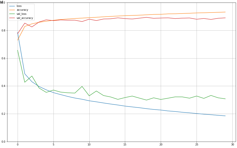

Loss and accuracy for our model

我们模型的损失和准确性

As can be seen above as the loss decreases, the accuracy increases. Two other things stand out from this plot:

从上面可以看出，随着损耗的减少，精度提高。 此情节还有另外两件事：

• We could probably train this model longer as it doesn’t look like the loss has reached a minimum
  我们可能会训练更长的时间，因为看起来损失似乎没有达到最小
• The accuracy of the training data set is higher than it is for the validation set (which is normal) but not wildly different to the validation dataset. This means there is no overfitting
  训练数据集的准确性高于验证集的准确性(这是正常的)，但与验证数据集没有太大不同。 这意味着没有过度拟合

评估神经网络的性能 (Evaluating the performance of the neural network)

Evaluating the performance of the network is straight forward and follows data science best practice principles. We call the model’s evalute method on the test data set to see how it performs. Remember that the test data set hasn’t been used in training and the network hasn’t seen this data before. We should perform this step only once so we can get an accurate idea of the model’s performance.

评估网络性能很简单，并且遵循数据科学最佳实践原则。 我们在测试数据集上调用模型的evalute方法，以查看其性能。 请记住，测试数据集尚未用于培训中，并且网络之前也没有看到过该数据。 我们应该只执行一次此步骤，这样我们才能对模型的性能有一个准确的了解。

model.evalute(X_test, y_test)

This will run the model on the test data set and the output should look something like this:

这将在测试数据集上运行模型，并且输出应如下所示：

313/313 [==============================] — 0s 2ms/step — loss: 0.3802 — accuracy: 0.8858

You’ll get an output of the loss and whatever other metrics specified when the model was compiled. Here we can see that this model is correct 88% of the time which isn’t bad for a simple network on such a difficult data set.

您将获得损失以及模型编译时指定的任何其他指标的输出。 在这里，我们可以看到该模型在88％的时间内都是正确的，对于在如此困难的数据集上的简单网络而言，这并不坏。

下一步 (Next steps)

In the next part of this series, I will talk about how to implement the above using a convolutional neural network and show how and why these perform better for image classification tasks.

在本系列的下一部分中，我将讨论如何使用卷积神经网络来实现上述内容，并展示这些方法如何以及为什么在图像分类任务中表现更好。

You can get the code I’ve used for this work from my Github here. Please bear in mind that it is a work in progress while I am writing these articles.

你可以和我已经用这项工作从我的Github上的代码在这里 。 请记住，在我撰写这些文章时，它正在进行中。

For part 3 of this series, I will link all of this back to my favourite passion outside data science, and that is SEO. How neural networks are using in search and what we can learn from them. Thanks for reading.

对于本系列的第3部分，我将把所有这些都链接到我最喜欢的数据科学之外的热情，那就是SEO。 神经网络如何在搜索中使用以及我们可以从中学到什么。 谢谢阅读。

翻译自: https://medium.com/@sandy_lee/how-to-train-neural-networks-for-image-classification-part-1-21327fe1cc1