python sqlite_python熊猫和sqlite

python sqlite

The SQLite database is a built-in feature of Python and a very useful one, at that. It is not a complete implementation of SQL but it has all the features that you need for a personal database or even a backend for a data-driven web site.

SQLite数据库是Python的内置功能，在那是非常有用的功能。 它不是SQL的完整实现，但具有个人数据库甚至数据驱动网站的后端所需的所有功能。

Using it with Pandas is simple and really useful. You can permanently store your dataframes in a table and read them directly into a new dataframe as you need them.

将它与Pandas一起使用非常简单，而且非常有用。 您可以将数据框永久存储在表中，并根据需要将它们直接读取到新数据框中。

But it isn’t just the storage aspect that is so useful. You can select and filter the data using simple SQL commands: this saves you having to process the dataframe itself.

但不仅仅是存储方面如此有用。 您可以使用简单SQL命令选择和过滤数据：这省去了处理数据框本身的麻烦。

I’m going to demonstrate a few simple techniques using SQLite and Pandas using my favourite London weather data set. It’s derived from public domain data from the UK Met Office and you can download it from my Github account.

我将使用我最喜欢的伦敦天气数据集演示一些使用SQLite和Pandas的简单技术。 它来自UK Met Office的公共领域数据，您可以从我的Github帐户下载它。

All the code here was written in a Jupyter notebook but should run perfectly well as a standalone Python program, too.

这里的所有代码都是在Jupyter笔记本中编写的，但也可以作为独立的Python程序完美运行。

Let’s start by importing the libraries:

让我们从导入库开始：

import sqlite3 as sql
import pandas as pd
import matplotlib.pyplot as plt

Obviously, we need the SQLite and Pandas libraries and we’ll get matplotlib as well because we are going to plot some graphs.

显然，我们需要SQLite和Pandas库，并且还将获得matplotlib，因为我们将绘制一些图。

Now let’s get the data. There’s about 70 years worth of temperature, rainfall and sunshine data in a csv file. We download it like this:

现在让我们获取数据。 CSV文件中包含大约70年的温度，降雨量和日照数据。 我们像这样下载它：

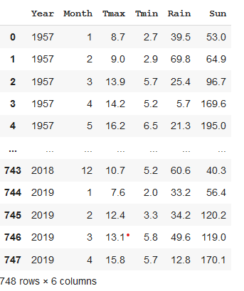
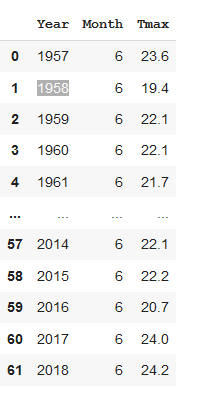
weather = pd.read_csv('https://github.com/alanjones2/dataviz/raw/master/londonweather.csv')

And this is what it looks like. The data is recorded for each month of the year. The temperatures are in degrees Celsius, the rainfall is in millimetres and ‘Sun’ is the total number of hours sunshine for the month.

这就是它的样子。 记录每年的每个月的数据。 温度以摄氏度为单位，降雨量以毫米为单位，“太阳”是该月阳光的总小时数。

Now we are going to save the dataframe in an SQLite database.

现在，我们将数据框保存在SQLite数据库中。

First we open a connection to a new database (this will create the database if it doesn’t already exist) and then create a new table in that database called weather.

首先，我们打开一个与新数据库的连接(如果尚不存在，它将创建一个数据库)，然后在该数据库中创建一个名为weather的新表。

conn = sql.connect('weather.db')
weather.to_sql('weather', conn)

We don’t need to run this code ever again unless the original data changes and, indeed, we shouldn’t, because SQLIte will not allow us to create a new table in the database if one of the same name already exists.

除非原始数据发生更改，否则我们无需再次运行此代码，并且实际上也不应更改该代码，因为如果已经存在同一个名称，SQLIte将不允许我们在数据库中创建新表。

Let’s assume that we have run the code above once and we have our database, weather, with the table, also called weather, in it. We could now start a new notebook or Python program to do the rest of this tutorial or simply comment out the code to download and create the database.

假设我们已经运行了上面的代码一次，并且在数据库中存储了weather，其中包含表(也称为weather )。 现在，我们可以启动一个新的Notebook或Python程序来完成本教程的其余部分，或者简单地注释掉要下载和创建数据库的代码。

So, we have a database with our weather data in it and now and we want to read it into a dataframe. Here is how we load the database table into a dataframe.

因此，我们现在和现在都有一个包含天气数据的数据库，我们希望将其读入数据框。 这是我们如何将数据库表加载到数据框中。

First, we make a connection to the database in the same way as before. Then we use the sql_read method from Pandas to read in the data. But to do this we have to send

首先，我们以与以前相同的方式建立到数据库的连接。 然后，我们使用Pandas中的sql_read方法读取数据。 但是要做到这一点，我们必须发送

a query to the database:

查询数据库：

SELECT * FROM weather

This is just about the simplest SQL query you can make. It means select all columns from the table called weather and return that data. Here’s the code (the query is passed as a string).

这只是您可以进行的最简单SQL查询。 这意味着从称为天气的表中选择所有列，然后返回该数据。 这是代码(查询以字符串形式传递)。

conn = sql.connect('weather.db')
weather = pd.read_sql('SELECT * FROM weather', conn)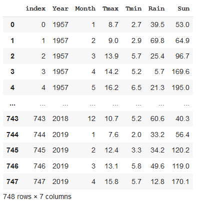

That, of course, is just reproducing the original dataframe, so let’s use the power of SQL to load just a subset of the data.

当然，那只是在复制原始数据帧，因此让我们使用SQL的功能仅加载一部分数据。

We’ll get the data for a couple of years, 50 years apart, and compare them to see if there was any clear difference.

我们将获得相隔50年的几年数据，并进行比较以查看是否存在明显差异。

Let’s start by getting the data for the year 2010.

让我们首先获取2010年的数据。

We are going to create a new dataframe called y2010 using read_sql, as before, but with a slightly different query. We add a WHERE clause. This only selects the data where the condition following the keyword WHERE is true. So, in this case, we only get the rows of data where the value in the year column is ‘2010’.

与以前一样，我们将使用read_sql创建一个名为y2010的新数据框，但查询略有不同。 我们添加一个WHERE子句。 仅选择关键字WHERE之后的条件为true的数据。 因此，在这种情况下，我们只获得year列中值为'2010'的数据行。

y2010 = pd.read_sql('SELECT * FROM weather WHERE Year == 2010', conn)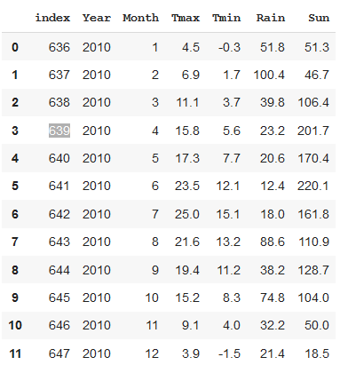

You can see that the only data that has been returned is for the year 2010.

您可以看到唯一返回的数据是2010年。

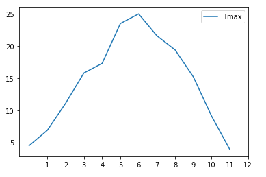
Here’s a line plot for Tmax.

这是Tmax的线图。

Now let’s do that again but for 1960, 50 years earlier

现在让我们再做一次，但在50年前的1960年

y1960 = pd.read_sql('SELECT * FROM weather WHERE Year == 1960', conn)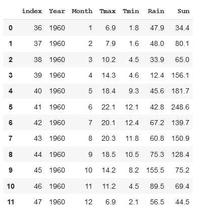

And now let’s plot the Tmax for the two individual years.

现在，让我们绘制两个年份的Tmax 。

ax2010 = y2010.plot(y='Tmax')
ax = y1960.plot(y='Tmax',color = 'red', ax=ax2010)
ax.legend(['2010','1960'])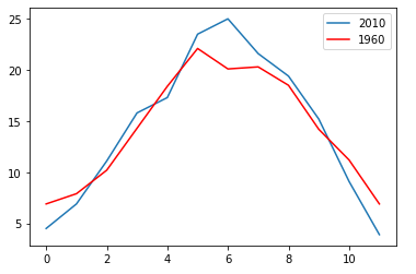

Interesting, 2010 was both hotter and colder than 1960 it seems. Is the weather getting more extreme? We need to do a bit more analysis to come to that conclusion.

有趣的是，2010年似乎比1960年更热更冷。 天气越来越极端了吗？ 我们需要做更多的分析才能得出结论。

Maybe we could start by finding the hottest years, say the ones where the temperature was over 25 degrees.

也许我们可以从找到最热的年份开始，比如温度超过25度的年份。

We do this by using a WHERE clause with a condition, Tmax > 25, that is, select the rows where Tmax was more than 25 degrees

通过使用条件为Tmax> 25的WHERE子句来执行此操作，即选择Tmax大于25度的行

But also since we are only interested in the max temperature, we will only select the columns that we are interested in. We do this by modifying the SELECT clause in the SQL query.

但是，由于我们只对最高温度感兴趣，因此我们将只选择我们感兴趣的列。我们通过修改SQL查询中的SELECT子句来做到这一点。

Instead of selecting * (i.e. all columns), we list the columns that we want returned: Year, Month and Tmax.

而不是选择*(即所有列)，而是列出要返回的列：Year，Month和Tmax。

high = pd.read_sql('SELECT Year,Month,Tmax FROM weather WHERE Tmax > 25', conn)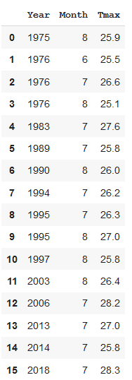

That’s in year order. Maybe it would be more interesting to have it in order of temperature.

这是按年顺序排列的。 按温度顺序排列也许会更有趣。

We can do that with SQL, too. We add the clause ORDER BY and give the column which should dictate the order. DESC means in descending order (omit that and you’ll get the default, ascending order).

我们也可以使用SQL来做到这一点。 我们添加子句ORDER BY并提供应指示顺序的列。 DESC表示按降序排列(忽略该名称，您将获得默认的升序排列)。

high = pd.read_sql('SELECT Year,Month,Tmax FROM weather WHERE Tmax > 25 ORDER BY Tmax DESC', conn)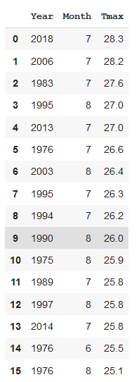

So, topping the chart is 2018 with 2006 not far behind. But 1983 and 1995 are in third and fourth place so there is no obvious pattern here that shows that temperatures are getting hotter over time.

因此，排在榜首的是2018年，紧随其后的是2006年。 但是1983年和1995年分别排在第三和第四位，因此这里没有明显的模式表明温度随着时间的推移变得越来越热。

One thing we can see is that the hottest months are in the summer! (Who’d have thought it.) But to be sure let’s plot a histogram.

我们可以看到的一件事是，最热的月份是夏天！ (谁会想到的。)但请确保我们绘制直方图。

high.plot.hist(y='Month', xticks=high['Month'])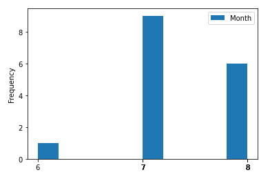

Yes, the hottest month tends to be July. So, if we are looking for a trend why don’t we take a look at the months of July throughout the decades and see how the temperature changes.

是的，最热的月份往往是七月。 因此，如果我们正在寻找趋势，为什么不回顾过去几十年的七月，看看温度是如何变化的。

Here’s another query:

这是另一个查询：

july = pd.read_sql('SELECT Year,Month,Tmax FROM weather WHERE month == 6', conn)

This gives us a table of temperature for all years but only where the month is equal to 6, i.e. July.

这为我们提供了所有年份的温度表，但仅当月份等于6时，即7月。

Now we’ll make a bar plot of the Tmax values over time.

现在，我们将绘制随时间变化的Tmax值的条形图。

july.plot.bar(x='Year', y='Tmax', figsize=(20,5));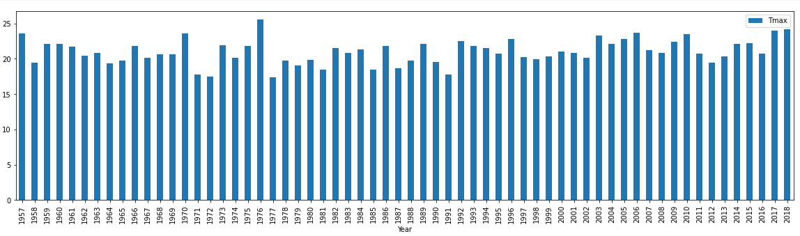

We could do a regression plot to see if there is any trend but frankly looking at this bar chart there is no obvious trend.

我们可以做一个回归图来查看是否存在任何趋势，但坦率地看一下该条形图没有明显的趋势。

So, with this extremely limited analysis of temperature data in London, we can’t come to any conclusion as to whether climate change is affecting Londoners (but from personal experience, I can tell that it’s feeling pretty warm there lately).

因此，通过对伦敦温度数据的分析极为有限，我们无法得出关于气候变化是否正在影响伦敦人的任何结论(但是根据个人经验，我可以告诉我最近那里的天气很温暖)。

But I hope that I’ve demonstrated that SQLite is a useful tool when used alongside Pandas and, if you haven’t done any SQL before, you can see how, even the tiny part of it that I’ve used here, might benefit your data analysis.

但是我希望我已经证明SQLite在与Pandas一起使用时是一个有用的工具，并且，如果您以前没有做过任何SQL，您可以看到，即使我在这里使用过的一小部分，也可能会受益。您的数据分析。

As always, thanks for reading.

与往常一样，感谢您的阅读。

And if you want to be informed about future articles please subscribe to my free newsletter.

如果您想了解以后的文章，请订阅我的免费新闻通讯。

翻译自: https://towardsdatascience.com/python-pandas-and-sqlite-a0e2c052456f

python sqlite