tidyverse清洗数据_通过使用Tidyverse挖掘性别平等数据获得的关键见解

最新推荐文章于 2024-04-09 14:59:37 发布

weixin_26737625

最新推荐文章于 2024-04-09 14:59:37 发布

阅读量279

点赞数

文章标签： python 大数据数据分析 java

原文链接：https://towardsdatascience.com/key-insights-obtained-by-mining-gender-equality-data-using-tidyverse-e9b80a557c72

版权

tidyverse清洗数据

Gender inequality is one of the most concerning areas which led the United Nations (UN) to set Sustainable Development Goal 5 — achieve gender equality and empower all women and girls. To assess the worldwide present day scenario, one of the best evaluation metrics is to rank the nation on the basis of the contribution of women in leadership and decision-making. To generate insights on the same ground, the `proportion of seats held by women in national parliaments (%)` can be considered as a foundational stone (data). The reason behind it is that in the present world, there are many regions where discriminatory laws and institutional practices are dominant to limit women’s capacity to run for political office. Systemic inequality, lack of access to education, limited options for workforce participation, and many other constraints on personal freedoms limit women from accessing the resources and opportunities to pursue a political career.

性别不平等是导致联合国(UN)制定可持续发展目标5—— 实现性别平等并赋予所有妇女和女孩权力的最令人关注的领域之一。为了评估当今世界范围内的情况，最好的评估指标之一是根据妇女在领导和决策中的贡献来对国家进行排名。为了从同一角度得出见解，可以将“妇女在国家议会中所占席位的比例(％)”视为基础(数据)。其背后的原因是，在当今世界上，许多地区的歧视性法律和体制惯例在很大程度上限制了妇女竞选政治职务的能力。系统性的不平等，缺乏受教育的机会，劳动力参与的选择有限以及对人身自由的许多其他限制，限制了妇女获得从事政治职业的资源和机会。

关于数据 (About Data)

The data source is a part of the Makeover Monday challenge (2020W30) and has been collated by The World Bank as part of their World Development Indicators database. The data reveals the country-wise proportion of seats held by women in national parliaments (%) at YoY Level (1997–2019). This data is part of the Visualize Gender Equality — Viz5 program.

该数据源是“ 改造星期一”挑战(2020W30)的一部分，并且已由世界银行整理为其“ 世界发展指标”数据库的一部分 。数据显示，妇女在国家议会中所占国家席位的比例(％)处于同比水平(1997-2019年)。此数据是“ 可视化性别平等-Viz5”程序的一部分。

探索性数据分析(EDA) (Exploratory Data Analysis (EDA))

The first step to generate insight out of data is to explore it. For this scenario, Tidyverse was used which is a key ingredient to do EDA in R. Following is the glimpse of data:

从数据中获得洞察力的第一步是对其进行探索。对于这种情况，使用了Tidyverse ，这是在R中进行EDA的关键因素。以下是数据的简要介绍：

head(Female_Political_Representation)Country.Name  Country.Code Year Proportion of Seats
1      Albania          ALB 1997                  NA
2      Albania          ALB 1998                  NA
3      Albania          ALB 1999          0.05161290
4      Albania          ALB 2000          0.05161290
5      Albania          ALB 2001          0.05714286
6      Albania          ALB 2002          0.05714286

For each country, we have Country Code, Year (1997–2019), and Proportion of seats held by women. From the glimpse, we can see that we have missing values {NA}.

对于每个国家/地区，我们都有国家/地区代码，年份(1997-2019年)和女性所占席位比例。从一瞥，我们可以看到我们缺少值{ NA} 。

Let’s check if missing values are at the initial year’s or at a random place.

让我们检查缺失值是在初始年份还是在随机位置。

missing_data <- filter(Female_Political_Representation, is.na(`Proportion of Seats`)) %>% # Filter only Missing values
  group_by(Year) %>%        # Group by Year
  summarise(count = n()) %>% # Count the instances
  arrange(desc(count))       # Arrange in descending order> missing_data
# A tibble: 20 x 2
    Year count
   <int> <int>
 1  1999    31
 2  1997    23
 3  2000    22
 4  2002    17
 5  1998    16
 6  2001    13
 7  2003     6
 8  2013     4
 9  2014     4
10  2017     3

As we can see, missing data is randomly distributed. Hence, for imputation we can follow two approaches:

如我们所见，丢失的数据是随机分布的。因此，为了推算，我们可以采用两种方法：

Capturing the individual country’s trend and using that to impute the missing years for that country.
捕捉单个国家的趋势，并以此来估算该国的缺失年份。
Using Forward Fill| Backward Fill method’s at the country level to impute missing value.
使用正向填充| 在国家/地区级别使用“ 后退填充”方法来估算缺失值。

I preferred the later one and used fill method by giving direction ‘downup’

我更喜欢后一种方法，并通过给定方向“ 向下 ”使用填充方法

Imputed_data <- Female_Political_Representation %>% 
                group_by(Country.Name,Country.Code) %>% # Group at Country Level
                fill(`Proportion of Seats`, .direction = "downup") # Missing Value Imputation  
  
colSums(is.na(Imputed_data)) # check for completeness

识别KPI (Identifying KPI)

The key objective after imputation is to identify how a particular country is effective in implementing gender-sensitive parliament — there is the freedom to women’s full participation. It can be assessed by computing a Year over Year (YoY) change in the proportion of women's seats. Following are the two metrics which can be created:

钥匙推算后的目标是确定一个特定国家如何有效实施对性别问题敏感的议会—妇女有充分参与的自由。可以通过计算女性席位比例的同比变化来评估。以下是可以创建的两个指标：

Difference vs Year Ago: It is obtained by subtracting a particular year’s value with a previous year’s value. It can be perceived as a means to compute lift — The more positive the difference, the better the country is in to implement awareness in gender equality. Also, we can rank the countries basis this metric.
差异与前一年的差异：通过将特定年份的价值减去上一年的价值而获得。可以将其视为计算升幅的一种方法-差异越积极，该国就越能更好地实现性别平等意识。同样，我们可以根据该指标对国家/地区进行排名。
Difference vs Start: It is obtained by computing the difference between present year proportion to the starting point. Formula : Proportion(2019) – Proportion(1997). The more positive the difference, the better the country has been improving towards gender-balanced representation across power structures and organizations.
差异与起点：通过计算当前比例与起点之间的差异获得。 公式：比例(2019)–比例(1997)。 差异越积极，该国在实现跨权力机构和组织的性别平衡代表制方面的改进就越好。

产生见解 (Generating Insights)

Using tidyverse, we can easily compute `Difference vs Year Ago` by using lag function.

使用tidyverse ，我们可以通过使用滞后函数轻松地计算“ 差异与年份 ” 。

# difference vs Year Ago Compute (At Country Level) ----KPI1 <- Imputed_data %>% 
         group_by(Country.Name,Country.Code) %>%mutate(Diff_vs_Year_Ago = 
`Proportion of Seats` - lag(`Proportion of Seats`)) %>% 
#Difference vs Year Ago fill(Diff_vs_Year_Ago, .direction = "downup") %>%  
# Missing Value Imputation  mutate(`Proportion of Seats` = round(`Proportion of Seats` *100,2),
Diff_vs_Year_Ago = round(Diff_vs_Year_Ago*100,2) 
# Data Standardization)

We can rank the country, to see at the yearly level, which country showed most improvement / least improvement.

我们可以对国家进行排名，以每年的水平查看哪个国家的进步最大/最小。

# Rank the differences at Yearly level ----
Rank1 <- KPI1 %>% 
         group_by(Year) %>% 
         mutate(rank = rank( - Diff_vs_Year_Ago, ties.method = "first"))

For 2019 (latest year), we can visualize top 10/ bottom 10 countries with the help of ggplot2 and plotly:

对于2019年(最新年)，我们可以借助ggplot2可视化排名前10位/排名前10位的国家， 并进行以下绘制 ：

library(plotly)
# Plot Top 10 Countries
top_10_plot <- Rank1 %>% 
  filter(Year == 2019 & rank < 11) %>% 
  ggplot(aes(x=reorder(Country.Name, `Proportion of Seats`), y= `Proportion of Seats`,fill = Country.Code)) +
  geom_bar(stat="identity")+
  theme_minimal() +
  theme(legend.position = "none")  +
  xlab("Country") + 
  coord_flip()# Convert to plotly
ggplotly(top_10_plot)

Image for post — Top 10 Countries (2019 vs 2018)

Story-point: Top 3 countries show that they are increasing proportion of seats greater than 10% as compared to last year, with UAE topping the list with 27.50%

故事点：排名前3位的国家/地区显示，与去年相比，他们的席位比例增加了10％以上，其中阿联酋以27.50％位居榜首

# Plot Bottom 10 Countries ----
bottom_10_plot <- Rank1 %>% 
  filter(Year == 2019 & rank >205) %>% 
  ggplot(aes(x=reorder(Country.Name, - Diff_vs_Year_Ago), y= Diff_vs_Year_Ago,fill = Country.Code)) +
  geom_bar(stat="identity")+
  theme_minimal() +
  theme(legend.position = "none")  +
  xlab("Country") + 
  coord_flip()# Convert to plotly
ggplotly(bottom_10_plot)

Story-point: All bottom10 countries show that they are declining at rate of less than 0% as compared to last year, with Tunisia topping the list with -8.7 %

故事要点：所有倒数10个国家/地区均显示，与去年相比下降幅度不到0％，突尼斯以-8.7％的优势位居榜首

Another perspective by which we can perform Top/Bottom analysis is to see how countries have evolved over time(‘Difference_vs_Starting point’). We can group at the country level and compute the difference of each instance with the starting year using ‘first’ method.

我们可以执行顶部/底部分析的另一个角度是观察国家随时间的变化情况( 'Difference_vs_Starting point' )。我们可以在国家/地区级别进行分组，并使用“第一”方法计算每个实例与开始年份的差异。

# Difference vs start Compute ----
KPI1 <- KPI1 %>%
  arrange(Year) %>%
  group_by(Country.Name) %>%
  mutate(Diff_vs_Start = `Proportion of Seats` - first(`Proportion of Seats`))# Compute Rank basis at Yearly Basis
Rank2 <- KPI1 %>% 
         group_by(Year) %>% 
         mutate(rank_Diff_vs_Start = rank( - Diff_vs_Start, ties.method = "first"))

For 2019 (latest year), we can visualize top 10/ bottom 10 countries positioning as follows:

对于2019年(最近一年)，我们可以将排名前10位/后10位的国家形象化，如下所示：

top_10_plot1 <- Rank2 %>% 
  filter(Year == 2019 & rank_Diff_vs_Start < 11) %>% 
  ggplot(aes(x=reorder(Country.Name, Diff_vs_Start), y= Diff_vs_Start,fill = Country.Code)) +
  geom_bar(stat="identity")+
  theme_minimal() +
  theme(legend.position = "none")  +
  xlab("Country") + 
  coord_flip()# Convert to plotly
ggplotly(top_10_plot1)

Story-point: Historically top 3 countries like UAE, Rwanda, and Bolivia indicate that they have shown an increase in the proportion of seats greater than 40 %, with UAE topping the list with 50%.

故事要点：历史上排名前3位的国家(如阿联酋，卢旺达和玻利维亚)表明，他们的席位比例增加了40％以上，其中阿联酋以50％的席位位居榜首。

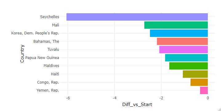
Story-point: Historically all bottom 10 countries follow decreasing trend at a rate of less than 0% as compared to the starting point, with Seychelles topping the list with -6.2 %

故事点：从历史上看，所有倒数第10个国家/地区的下降趋势均低于起点，且下降幅度小于0％，塞舌尔以-6.2％的优势位居榜首

** Global Level Insights —

**全球层面的见解-

From the perspective of the global level performance, we can group the data at a yearly level, ignoring countries and get the revised KPI’s as follows:

从全球绩效的角度来看，我们可以按年度级别对数据进行分组，而忽略国家/地区，并获得修订后的KPI，如下所示：

# Global Level Trend ----
Global_Insight <- KPI1 %>% 
                  group_by(Year) %>% 
                  summarize(
                    Avg_Proportion_of_Seats = mean(`Proportion of Seats`),
                    Avg_Diff_vs_Year_Ago = mean(Diff_vs_Year_Ago),
                    Avg_Diff_vs_Start = mean(Diff_vs_Start)
                    
                  )> mean(Global_Insight$Avg_Diff_vs_Year_Ago) # Compute Average Lift
0.5781982##########################################################Year Avg_Proportion_of_Seats
   <int>                   <dbl>
 1  1997                    10.4
 2  1998                    10.8
 3  1999                    11.2 
 ----------------------------------
 4  2017                    21.9  
 5  2018                    22.5  
 6  2019                    23.3
##########################################################

Also, we can use this data to create an area plot, which will showcase the global trend as shown in the code below:

同样，我们可以使用此数据来创建面积图，该面积图将展示全局趋势，如以下代码所示：

# Area plot ----# Plot 1
Avg_Proportion_of_Seats_plot <-  ggplot(Global_Insight, aes(x = Year, y = Avg_Proportion_of_Seats)) + 
  geom_area(fill ="#00AFBB", alpha = 0.5, position = position_dodge(0.8))ggplotly(Avg_Proportion_of_Seats_plot)# Plot 2
Avg_Diff_vs_Year_Ago_plot <-  ggplot(Global_Insight, aes(x = Year, y = Avg_Diff_vs_Year_Ago)) + 
  geom_area(fill ="#ff7a00", alpha = 0.5, position = position_dodge(0.8))ggplotly(Avg_Diff_vs_Year_Ago_plot)# Plot 3
Avg_Diff_vs_Start_plot <-  ggplot(Global_Insight, aes(x = Year, y = Avg_Diff_vs_Start)) + 
  geom_area(fill ="#0dff00", alpha = 0.5, position = position_dodge(0.8))ggplotly(Avg_Diff_vs_Start_plot)# Combine 3 plots ----
library(ggpubr)
theme_set(theme_pubr())figure <- ggarrange(Avg_Proportion_of_Seats_plot, Avg_Diff_vs_Year_Ago_plot, Avg_Diff_vs_Start_plot,
                    labels = c("Avg_Proportion_of_Seats", "Avg_Diff_vs_Year_Ago", "Avg_Diff_vs_Start"),
                    ncol = 1, nrow = 3)figure

Story-point: As we can see, the proportion of seats at a global level went high from 10.4% (1997) to 23.3% (2019), with an average lift of 0.57% per year. Also, the Diff_vs_Year_Ago is following peaks and valleys with the highest increase in 2007 and the lowest dip in 2010

故事点：正如我们所看到的，全球席位比例从1997年的10.4％上升到2019年的23.3％，平均每年提升0.57％ 。 此外，Diff_vs_Year_Ago紧随高峰和低谷，其增幅在2007年最高，在2010年最低

尾注 (End Notes)

This insight generation journey started with exploring and cleaning data, standardizing it (missing value imputation), identifying KPI’s, creating effective visuals to answer questions, and telling a meaningful story out of it. Also, tidyverse comes in quick handy for mining insights from data which can later be integrated to tableau public to create quick visuals and story-line as shown below:

这一洞察力的生成过程始于探索和清理数据，对其进行标准化(缺失价值估算)，识别KPI，创建有效的视觉效果以回答问题并从中讲出有意义的故事。此外， tidyverse可以快速方便地从数据中挖掘见解，随后可以将其集成到Tableau公众中，以创建快速的视觉效果和故事情节 ，如下所示：

Forecast from the above figure is indicating that by 2030, women's proportion in the political role is contributing to only 27.67%, as opposed to United Nation’s target of reaching 50%.

根据以上数字预测，到2030年 ，妇女在政治角色中的比例仅占27.67％，而联合国的目标是达到50％。

Link to Tableau Public dashboard: link

链接到 Tableau Public仪表板： 链接

Link to code and visuals: link

链接到代码和视觉效果：链接