高光谱图像分类_高光谱图像分析-分类-CSDN博客

本文探讨了高光谱图像的分类技术，主要聚焦于数据处理和机器学习方法在高光谱图像分析中的应用。内容涉及从原始数据到分类结果的全过程，包括图像预处理、特征选择和使用Python、机器学习及人工智能算法进行分类。

摘要由CSDN通过智能技术生成

高光谱图像分类

初学者指南 (Beginner’s Guide)

This article provides detailed implementation of different classification algorithms on Hyperspectral Images(HSI).

本文提供了在高光谱图像(HSI)上不同分类算法的详细实现。

目录 (Table of Contents)

Introduction to Hyperspectral Images(HSI)
高光谱图像(HSI)简介
Dimensionality Reduction(DR)
降维(DR)
Classification Algorithms
分类算法
Implementation — Classification on HSI
实施-恒指分类

高光谱图像(HSI)简介 (Introduction to Hyperspectral Images(HSI))

In Remote Sensing, Hyperspectral remote sensors are widely used for monitoring the earth’s surface with the high spectral resolution. Generally, the HSI contains more than three bands compared to conventional RGB Images. The Hyperspectral Images(HSI) are used to address a variety of problems in diverse areas such as Crop Analysis, Geological Mapping, Mineral Exploration, Defence Research, Urban Investigation, Military Surveillance, etc.

在遥感中 ，高光谱遥感器广泛用于以高光谱分辨率监视地球表面。通常，与传统的RGB图像相比，HSI包含三个以上的波段。高光谱图像(HSI)用于解决作物分析， 地质制图 ， 矿物勘探 ， 国防研究，城市调查，军事监视等各个领域的各种问题。

Use the below article which provides information on Data Collection, Data Preprocessing, and Exploratory Data Analysis on HSI.

使用下面的文章，它提供有关HSI上的数据收集 ， 数据预处理和探索性数据分析的信息。

There are various open-source sites providing hyperspectral data for learning purposes. Here are the two popular sites:

有许多开放源站点提供高光谱数据用于学习目的。这是两个受欢迎的网站：

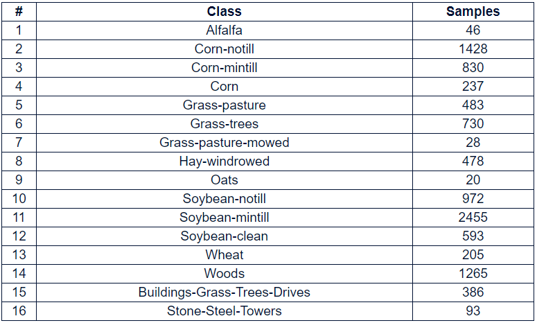
In this article, we use the Indian Pines(IP) Hyperspectral Image Dataset. The Indian Pines(IP) HSI data is gathered using the AVIRIS sensor over the Indian Pines test site in North-western Indiana and it consists of 145 X 145 pixels, 16 classes, and 200 bands. Here are the Ground Truth details of the Indian Pines(IP) Dataset:

在本文中，我们使用“ 印度松(IP)高光谱图像数据集”。印度派恩斯(IP)HSI数据是使用AVIRIS传感器在印第安纳州西北部的印度派恩斯测试站点上收集的，它由145 X 145像素，16个类别和200个波段组成。以下是印度松树(IP)数据集的地面真相详细信息：

Image for post — Ground Truth Details of Indian Pines(IP) Dataset

The code to read the dataset:

读取数据集的代码：

from scipy.io import loadmat


def read_HSI():
  X = loadmat('Indian_pines_corrected.mat')['indian_pines_corrected']
  y = loadmat('Indian_pines_gt.mat')['indian_pines_gt']
  print(f"X shape: {X.shape}\ny shape: {y.shape}")
  return X, y


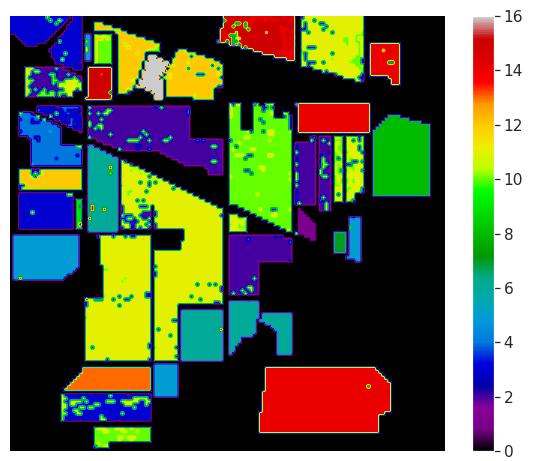
X, y = read_HSI()

The visualization of the Ground Truth of the Indian Pines dataset is shown below:

印度松树数据集的地面真相的可视化如下所示：

The visualization of the six randomly selected bands over 200 is shown below:

下面显示了200多个随机选择的六个波段的可视化：

降维(DR) (Dimensionality Reduction(DR))

Dimensionality Reduction is used to reduce the number of dimensions of the data, thereby paving the way for the classifiers to generate comprehensive models at a low computational cost. Hence, Dimensionality Reduction (DR) has become more prominent to improve the accuracy of pixel classification in Hyperspectral Images(HSI).

降维用于减少数据的维数，从而为分类器以较低的计算成本生成综合模型铺平了道路。因此，降维(DR)在提高高光谱图像(HSI)中像素分类的准确性方面变得更加突出。

Dimensionality Reduction can be done in two types. They are:

降维可以采用两种类型。他们是：

Feature Selection
功能选择
Feature Extraction
特征提取

Feature Selection is the process of selecting dimensions of features of the dataset which contributes mode to the machine learning tasks such as classification, clustering, e.t.c. This can be achieved by using different methods such as correlation analysis, univariate analysis, e.t.c.

特征选择是选择数据集特征维度的过程，该特征维度有助于机器学习任务的模式，例如分类，聚类等。这可以通过使用不同的方法(例如相关分析，单变量分析等)来实现

Feature Extraction Feature Extraction is a process of finding new features by selecting and/or combining existing features to create reduced feature space, while still accurately and completely describing the data set without loss of information.

特征提取特征提取是通过选择和/或组合现有特征以创建缩小的特征空间来查找新特征的过程，同时仍能准确，完整地描述数据集而不会丢失信息。

Based on the criterion function and process of convergence, dimensionality reduction techniques are also classified as Convex and Non-Convex. Some popular dimensionality reduction techniques include PCA, ICA, LDA, GDA, Kernel PCA, Isomap, Local linear embedding(LLE), Hessian LLE, etc.

基于准则函数和收敛过程，降维技术也分为凸和非凸。一些流行的降维技术包括PCA，ICA，LDA，GDA，内核PCA，Isomap，局部线性嵌入(LLE)，Hessian LLE等。

Use the below article “Dimensionality Reduction in Hyperspectral Images using Python” to get a better understanding.

使用下面的文章“使用Python减少高光谱图像的维数”以获得更好的理解。

In this article, we are going to use Principal Component Analysis(PCA) to reduce the dimensionality of the data.

在本文中，我们将使用主成分分析(PCA)来减少数据的维数。

主成分分析(PCA) (Principal Component Analysis(PCA))

Principal Component Analysis(PCA) is one of the standard algorithms used to reduce the dimensions of the data. PCA is a non-parametric algorithm that increases the interpretability at the same time reducing the minimizing the loss of information(Reconstruction Error).

主成分分析(PCA)是用于减少数据量的标准算法之一。 PCA是一种非参数算法，可在提高解释性的同时减少信息损失(重构错误)。

Use the below two papers for better understanding the math behind the PCA.

使用以下两篇论文可以更好地理解PCA背后的数学原理。

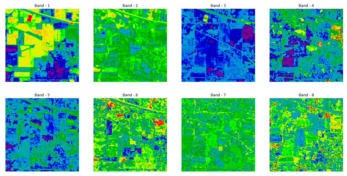
Based on the explained variance ratio the number of components is taken as 40. The below code explains —

根据解释的方差比，组件个数为40。以下代码说明了-

pca = PCA(n_components = 40)


dt = pca.fit_transform(df.iloc[:, :-1].values)


q = pd.concat([pd.DataFrame(data = dt), pd.DataFrame(data = y.ravel())], axis = 1)


q.columns = [f'PC-{i}' for i in range(1,41)]+['class']

The first eight principal components or eight bands are shown below:

前八个主要成分或八个频段如下所示：

分类算法 (Classification Algorithms)

Classification refers to a predictive modeling problem where a class label is predicted for the given input data. The classification can be divided as :

分类是指预测建模问题，其中针对给定输入数据预测类别标签。分类可分为：

Classification Predictive Modeling
分类预测建模
Binary Classification
二进制分类
Multi-Class Classification
多类别分类
Multi-Label Classification
多标签分类
Imbalanced Classification
分类不平衡

Today, we are dealing with the Multi-Class Classification problem. There are different classification algorithms that are used for the classification of Hyperspectral Images(HSI) such as :

今天，我们正在处理“多类分类”问题。高光谱图像(HSI)的分类有不同的分类算法，例如：

K-Nearest Neighbors
K最近邻居
Support Vector Machine
支持向量机
Spectral Angle Mapper
光谱角映射器
Convolutional Neural Networks
卷积神经网络
Decision Trees e.t.c
决策树等

In this article, we are going to use the Support Vector Machine(SVM) to classify the Hyperspectral Image(HSI).

在本文中，我们将使用支持向量机(SVM)对高光谱图像(HSI)进行分类。

支持向量机(SVM) (Support Vector Machine(SVM))

Support Vector Machine is a supervised classification algorithm that maximizes the margin between data and hyperplane. Different kernel functions are used to project the data into higher dimensions such as Linear, polynomial, Radial Basis Function(RBF), e.t.c.

支持向量机是一种监督分类算法，可最大化数据和超平面之间的余量。使用不同的内核函数将数据投影到更高的维度，例如线性，多项式，径向基函数(RBF)等

For better understanding, the concept behind SVM refer the below lectures:

为了更好地理解，SVM背后的概念请参考以下讲座：

实施-恒指分类 (Implementation — Classification on HSI)

The below code serves the purpose of implementing the support vector machine to classify the Hyperspectral Image.

以下代码用于实现支持向量机以对高光谱图像进行分类的目的。

x = q[q['class'] != 0]


X = x.iloc[:, :-1].values


y = x.loc[:, 'class'].values 


names = ['Alfalfa',	'Corn-notill', 'Corn-mintill',	'Corn',		'Grass-pasture','Grass-trees',
'Grass-pasture-mowed','Hay-windrowed','Oats','Soybean-notill','Soybean-mintill',
'Soybean-clean', 'Wheat',	'Woods',	'Buildings Grass Trees Drives',	'Stone Steel Towers']


X_train, X_test, y_train, y_test = train_test_split(X, y, test_size=0.20, random_state=11, stratify=y)


svm =  SVC(C = 100, kernel = 'rbf', cache_size = 10*1024)


svm.fit(X_train, y_train)


ypred = svm.predict(X_test)

The confusion matrix is generated using the code:

混淆矩阵是使用以下代码生成的：

data = confusion_matrix(y_test, ypred)


df_cm = pd.DataFrame(data, columns=np.unique(names), index = np.unique(names))


df_cm.index.name = 'Actual'


df_cm.columns.name = 'Predicted'


plt.figure(figsize = (10,8))


sn.set(font_scale=1.4)#for label size


sn.heatmap(df_cm, cmap="Reds", annot=True,annot_kws={"size": 16}, fmt='d')


plt.savefig('cmap.png', dpi=300)

The generated Classification Report which consists of the Classwise Accuracy, Accuracy Precision, Recall, F1 Score, and Support is shown below:

生成的分类报告由分类准确性，准确性准确性，召回率，F1得分和支持组成，如下所示：

Finally, the classification Map is shown below:

最后，分类图如下所示：

The entire code that I have written in this article can be accessed using the below notebook in GitHub and CoLab.

可以使用GitHub和CoLab中的以下笔记本访问本文中编写的全部代码。