


已知两点坐标拾取怎么操作
有关深层学习的FAU讲义 (FAU LECTURE NOTES ON DEEP LEARNING)
These are the lecture notes for FAU’s YouTube Lecture “Deep Learning”. This is a full transcript of the lecture video & matching slides. We hope, you enjoy this as much as the videos. Of course, this transcript was created with deep learning techniques largely automatically and only minor manual modifications were performed. Try it yourself! If you spot mistakes, please let us know!
这些是FAU YouTube讲座“ 深度学习 ”的 讲义 。 这是演讲视频和匹配幻灯片的完整记录。 我们希望您喜欢这些视频。 当然,此成绩单是使用深度学习技术自动创建的,并且仅进行了较小的手动修改。 自己尝试! 如果发现错误,请告诉我们!
导航 (Navigation)
Previous Lecture / Watch this Video / Top Level
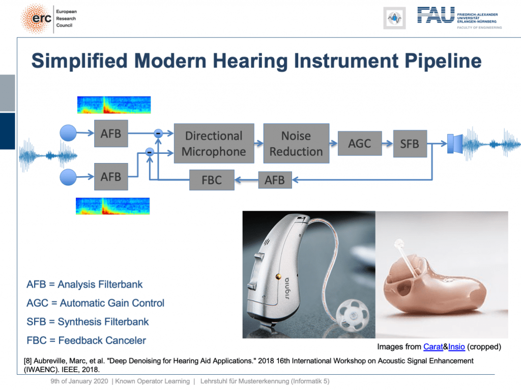
Welcome back to deep learning! This is it. This is the final lecture. So today, I want to show you a couple of more applications of this known operator paradigm and also some ideas where I believe future research could actually go to. So, let’s see what I have here for you. Well, one thing that I would like to demonstrate is the simplified modern hearing aid pipeline. This is a collaboration with a company that is producing hearing aids and they typically have a signal processing pipeline where you have two microphones. They collect some speech signals. Then, this is run through an analysis filter bank. So, this is essentially a short-term Fourier transform. This is then run through a directional microphone in order to focus on things that are in front of you. Then, you use noise reduction in order to get better intelligibility for the person who is wearing the hearing aid. This is followed by an automatic gain control and using the gain control you then do a synthesis of the frequency analysis back to a speech signal that is then played back on a loudspeaker within the hearing aid. So, there’s also a recurrent connection because you want to suppress feedback loops. This kind of pipeline, you can find in modern-day hearing aids of various manufacturers. Here, you see some examples and the key problem in all of this processing is here the noise reduction. This is the difficult part. All the other things, we know how to address with traditional signal processing. But the noise reduction is something that is a huge problem.
欢迎回到深度学习! 就是这个。 这是最后的演讲。 因此,今天,我想向您展示这个已知的运算符范例的更多应用程序,以及一些我认为将来可以进行实际研究的想法。 所以,让我们看看我在这里为您准备的。 好吧,我想展示的一件事是简化的现代助听器管道。 这是与一家生产助听器的公司的合作,它们通常具有信号处理管道,其中有两个麦克风。 他们收集一些语音信号。 然后,将其运行通过分析过滤器库。 因此,这本质上是短期傅立叶变换。 然后将其通过定向麦克风运行,以专注于前方的事物。 然后,您可以使用降噪功能来使佩戴助听器的人获得更好的清晰度。 接下来是自动增益控制,然后使用增益控制将频率分析合成为语音信号,然后在助听器内的扬声器上播放语音信号。 因此,还有一个循环连接,因为您要抑制反馈循环。 您可以在各种制造商的现代助听器中找到这种管道。 在这里,您会看到一些示例,所有这些处理过程中的关键问题是噪声的降低。 这是困难的部分。 所有其他的事情,我们知道如何用传统的信号处理解决。 但是降噪是一个很大的问题。
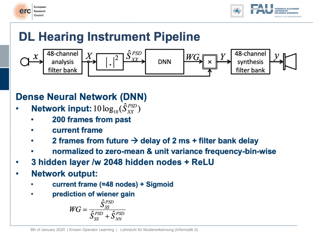
So, what can we do? Well, we can map this entire hearing aid pipeline onto a deep network. Onto a deep recurrent network and all of those steps can be expressed in terms of differentiable operations.
所以,我们能做些什么? 好吧,我们可以将整个助听器管道映射到一个深层网络。 进入深度循环网络,所有这些步骤都可以通过可区分的操作来表示。
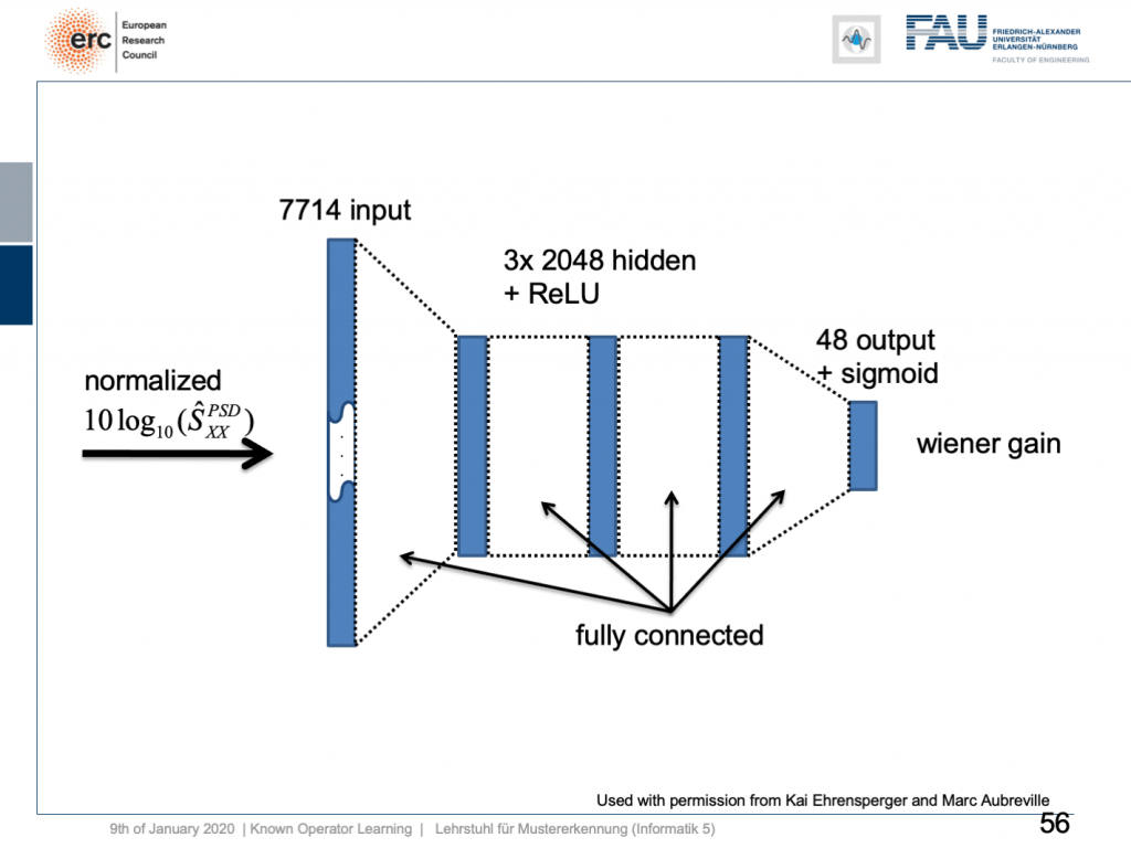
If we do so, we set up the following outline. Actually, our network here is not so deep because we only have three hidden layers but with 2024 hidden nodes and ReLUs. This is then used to predict the coefficients of a Wiener filter gain in order to suppress channels that have particular noises. So, this is the setup. We have an input of seven thousand seven hundred and fourteen nodes from our normalized spectrum. Then, this is run through three hidden layers. They are fully connected with ReLUs and in the end, we have some output that is 48 channels produced by the sigmoid producing our Wiener gain.
如果这样做,我们将建立以下概述。 实际上,我们的网络并不那么深,因为我们只有三个隐藏层,但有2024个隐藏节点和ReLU。 然后将其用于预测维纳滤波器增益的系数,以便抑制具有特定噪声的通道。 因此,这就是设置。 从归一化频谱中,我们输入了77414个节点。 然后,这将贯穿三个隐藏层。 它们与ReLU完全相连,最后,我们的输出是由S型产生的48个通道,产生了我们的维纳增益。
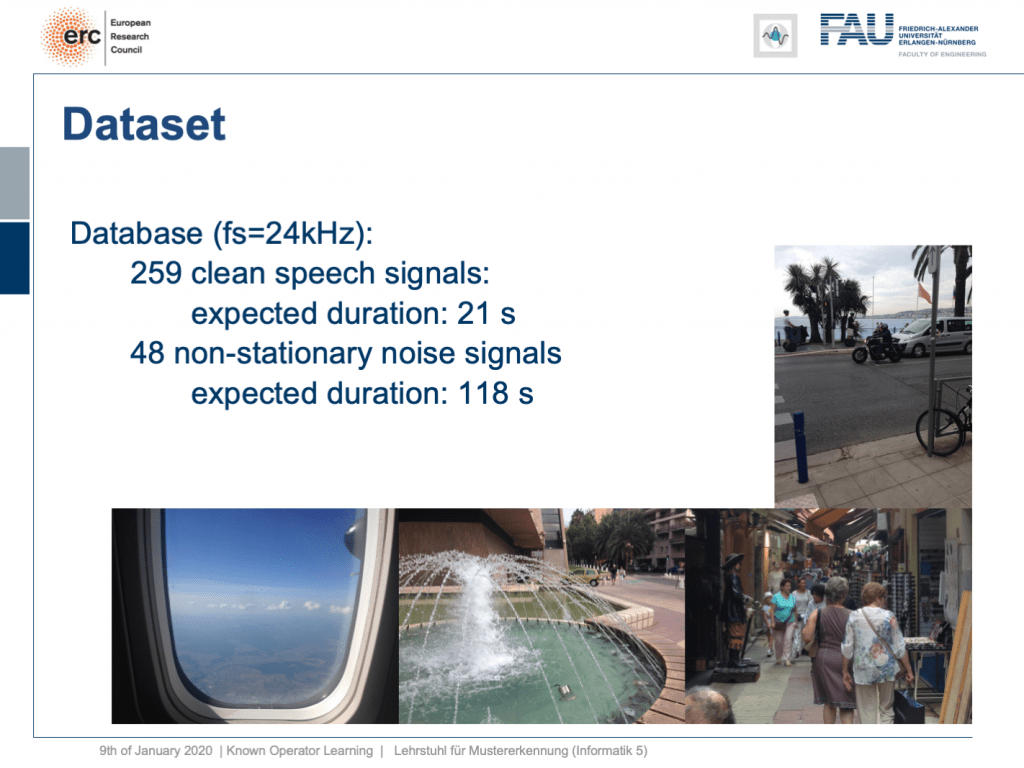
We evaluated this on some data set and here we had 259 clean speech signals. We then essentially had 48 non-stationary noise signals and we mixed them. So, you could argue what we’re essentially training here is a kind of recurrent autoencoder. Actually, a denoising autoencoder because as input we take the clean speech signal plus the noise and on the output, we want to produce the clean speech signal. Now, this is the example.
我们在一些数据集上对此进行了评估,这里有259个干净的语音信号。 然后,我们基本上得到了48个非平稳噪声信号,并对其进行了混合。 因此,您可以争辩说,我们在这里实际上要训练的是一种递归自动编码器。 实际上,是一种去噪自动编码器,因为我们将干净的语音信号加噪声作为输入,并在输出上要产生干净的语音信号。 现在,这是示例。
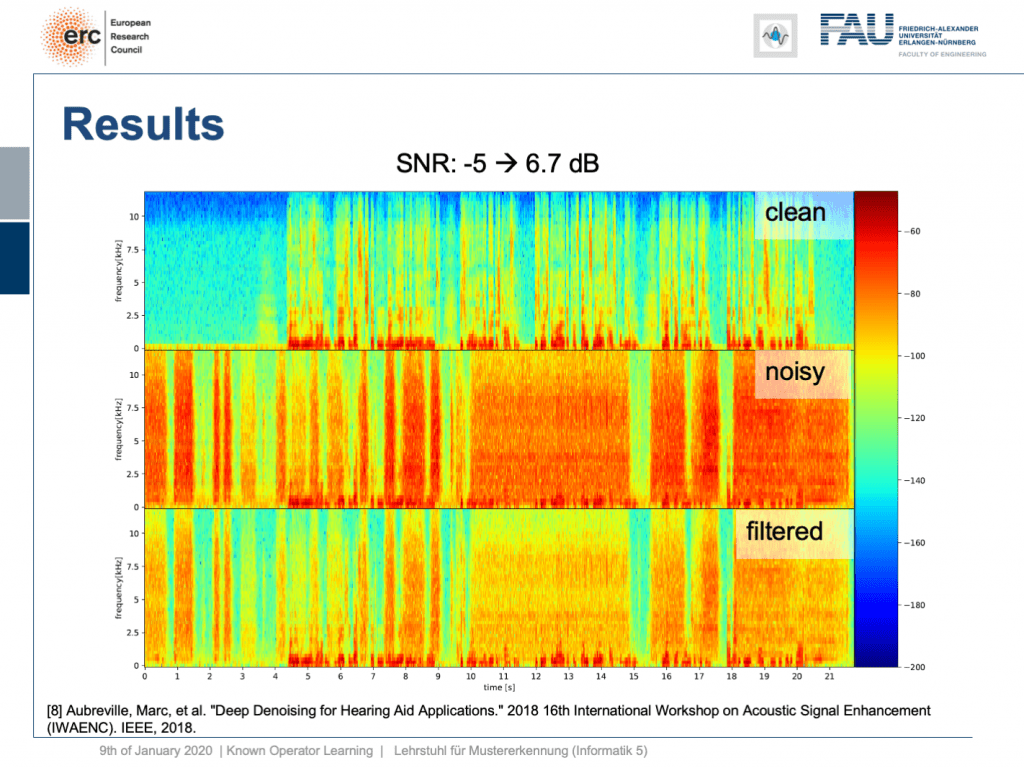
Let’s try a non-stationary noise pattern and this is an electronic drill. Also, note that the network has never heard an electronic drill before. This typically kills your hearing aid and let’s listen to the output. So, you can hear that the non-stationary noise is also very well suppressed. Wow. So, that’s pretty cool of course there are many more applications of this.
让我们尝试一个非平稳的噪声模式,这是一个电钻。 另外,请注意,网络之前从未听过电子演习。 这通常会杀死您的助听器,让我们听听输出。 因此,您会听到非平稳噪声也得到了很好的抑制。 哇。 因此,这很酷,当然还有更多的应用程序。

Let’s look into one more idea. Can we derive networks? So here, let’s say you have a scenario where you collect data in a format that you don’t like, but you know the formal equation between the data and the projection.
让我们再看看一个想法。 我们可以得出网络吗? 因此,在这里,假设您有一个场景,其中以您不喜欢的格式收集数据,但是您知道数据和投影之间的形式方程式。
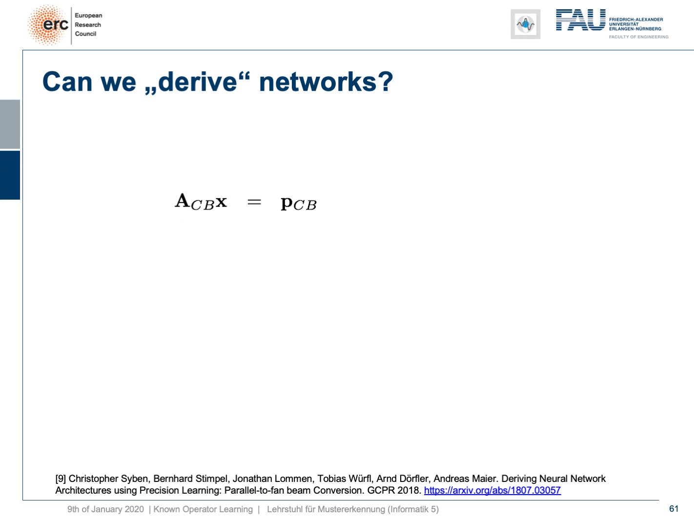
So, the example that I’m showing here is a cone-beam acquisition. This is simply a typical x-ray geometry. So, you take an X-ray and this is typically conducted in cone-beam geometry. Now, for the cone-beam geometry, we can describe it entirely using this linear operator as we’ve already seen in the previous video. So, we can express the relation between the object x our geometry A subscript CB and our projection p subscript CB. Now, the cone-beam acquisition is not so great because you have magnifications in there. So if you have something close to the source, it will be magnified more than an object closer to the detector. So, this is not so great for diagnosis. In othopedics, they would prefer parallel projections because if you have something, it will be orthogonally projected and it’s not magnified. This would be really great for diagnosis. You would have metric projections and you can simply measure int the projection and it would have the same size as inside the body. So, this would be really nice for diagnosis, but typically we can’t measure it with the systems that we have. So, in order to create this, you would have to create a full reconstruction of the object, doing a full CT scan from all sides, and then reconstruct the object and project it again. Typically in orthopedics, people don’t like slice volumes because they are far too complicated to read. But projection images are much nicer to read. Well, what can we do? We know the factor that connects two equations here is x. So we can simply solve this equation here and produce the solution with respect to x. Once, we have x and the matrix inverse here of A subscript CB times p subscript CB. Then, we simply would multiply it to our production image. But we are not interested in the reconstruction. We are interested in this projection image here. So, let’s plug it into our equation and then we can see that by applying this series of matrices we can convert our cone-beam projections into a parallel-beam projection p subscript PB. There’s no real reconstruction required. Only a kind of intermediate reconstruction is required. Of course, you don’t just acquire a single projection here. You may want to acquire a couple of those projections. Let’s say three or four projections but not thousands as you would in a CT scan. Now, if you look at this set of equations, we know all of the operations. So, this is pretty cool. But we have this inverse here and note that this is again a kind of reconstruction problem, an inverse of a large matrix that is sparse to a large extent. So, we still have a problem estimating this guy here. This is very expensive to do, but we are in the world of deep learning and we can just postulate things. So, let’s postulate that this inverse is simply a convolution. So, we can replace it by a Fourier transform a diagnoal matrix K and an inverse Fourier transform. Suddenly, I’m only estimating parameters of a diagonal matrix which makes the problem somewhat easier. We, can solve it in this domain and again we can use our trick that we have essentially defined a known operator net topology here. We can simply use it with our neural network methods. We use the backpropagation algorithm in order to optimize this guy here. We just use the other layers as fixed layers. By the way, this could also be realized for nonlinear formulas. So, remember as soon as we’re able to compute a subgradient, we can plug it into our network. So you can also do very sophisticated things like including a median filter for example.
因此,我在这里显示的示例是一个锥束采集。 这只是典型的X射线几何形状。 因此,您需要拍摄X射线,并且通常以锥形束几何形状进行。 现在,对于锥束几何形状,我们可以完全使用此线性运算符对其进行描述,就像我们在上一个视频中已经看到的那样。 因此,我们可以表示对象x我们的几何A下标CB和我们的投影p下标CB之间的关系。 现在,锥束采集不是那么好,因为那里有放大倍数。 因此,如果您靠近源头,它会比靠近探测器的对象被放大。 因此,这对于诊断不是那么好。 在骨科手术中,他们更喜欢平行投影,因为如果您有东西,它将被正交投影并且不会被放大。 这对于诊断确实非常有用。 您将拥有公制投影,并且您可以简单地测量int投影,它的尺寸将与人体内部相同。 因此,这对于诊断确实非常好,但是通常我们无法使用已有的系统对其进行测量。 因此,为了创建此对象,您将必须创建对象的完整重建,从各个侧面进行完整的CT扫描,然后重建对象并再次对其进行投影。 通常在整形外科中,人们不喜欢切片,因为它们太复杂而难以阅读。 但是投影图像更易于阅读。 好吧,我们该怎么办? 我们知道这里连接两个方程的因数是x 。 因此,我们可以在这里简单地求解此方程,并产生关于x的解。 一次,我们有x和A下标CB乘以p下标CB的矩阵逆。 然后,我们只需将其乘以我们的生产图像即可。 但是我们对重建不感兴趣。 我们对此投影图像感兴趣。 因此,让我们将其插入方程式中,然后我们可以看到,通过应用这一系列矩阵,我们可以将锥束投影转换为平行束投影p下标PB。 不需要真正的重建。 仅需要一种中间重建。 当然,您不仅在这里获得了一个投影。 您可能需要获得其中的一些预测。 假设有3或4个投影,但不像CT扫描中的投影那样成千上万个。 现在,如果您查看这组方程,我们知道所有操作。 因此,这非常酷。 但是我们在这里有这个逆,并注意到这又是一种重构问题,是在很大程度上稀疏的大矩阵的逆。 因此,在此估算这个人仍然有问题。 这样做非常昂贵,但是我们处在深度学习的世界中,我们只能假设一些事情。 因此,我们假设该逆只是卷积。 因此,我们可以用诊断矩阵K和傅立叶逆变换进行傅立叶变换来代替它。 突然,我只是估计对角矩阵的参数,这使问题更容易解决。 我们可以在此域中解决它,并且再次可以使用我们的技巧,即在这里本质上定义了已知的操作员网络拓扑。 我们可以简单地将其与我们的神经网络方法一起使用。 我们在这里使用反向传播算法来优化此人。 我们只是将其他层用作固定层。 顺便说一下,这对于非线性公式也可以实现。 因此,请记住,一旦我们能够计算出次梯度,就可以将其插入我们的网络。 因此,您还可以做一些非常复杂的事情,例如包括一个中值滤波器。
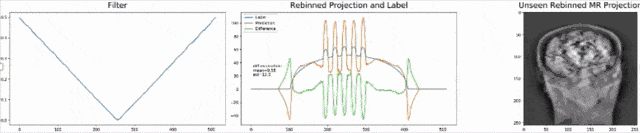
Let’s look at an example here. We do the rebinning of MR projections in this case. We will do an acquisition in k-space and these are typically just parallel projections. Now, we’re interested in generating overlay for X-rays and x-rays we need the come-beam geometry. So, we take a couple of our projections and then rebin them to match exactly the come-beam geometry. The cool thing here is that we would be able to unite the contrasts from MR and X-ray in a single image. This is not straightforward. If you initialize with just the Ram-Lak filter, what you would get is the following thing here. So in this plot here, you can see the difference between the prediction and the ground truth in green, the ground truth or label is shown in blue, and our prediction is shown in orange. We trained only on geometric primitives here. So, we train with a superposition of cylinders and some Gaussian noise, and so on. There is never anything that even looks faintly like a human in the training data set, but we take this and immediately apply it to an anthropomorphic phantom. This is to show you the generality of the method. We are estimating very few coefficients here. This allows us very very nice generalization properties onto things that have never been seen in the training data set. So, let’s see what happens over the iterations. You can see the filter deforms and we are approaching, of course, the correct label image here. The other thing that you see is that this image on the right got dramatically better. If I go ahead with a couple of more iterations, you can see we can really get a crisp and sharp image. Obviously, we can also not just in look into a single filter, but instead individual filters for the different parallel projections.
让我们在这里看一个例子。 在这种情况下,我们将对MR投影进行重新组合。 我们将在k空间中进行采集,这些通常只是平行投影。 现在,我们对生成X射线和X射线的叠加层感兴趣,我们需要光束几何。 因此,我们采用了几个投影,然后重新组合它们以完全匹配光束几何。 这里很酷的事情是,我们将能够将MR和X射线的对比度合并到一个图像中。 这并不简单。 如果仅使用Ram-Lak过滤器进行初始化,那么您将获得以下内容。 因此,在此图中,您可以看到预测与绿色之间的差异,绿色或蓝色显示地面预测或标签,橙色显示我们的预测。 在这里,我们仅对几何图元进行训练。 因此,我们用圆柱体和一些高斯噪声的叠加进行训练,等等。 在训练数据集中,从来没有任何东西看起来像人一样微弱,但是我们接受了这一点,并立即将其应用于拟人化模型。 这是向您展示该方法的一般性。 在这里,我们估计的系数很小。 这使我们对训练数据集中从未见过的事物具有非常好的泛化属性。 因此,让我们看看在迭代过程中会发生什么。 您会看到过滤器变形,我们当然在这里接近正确的标签图像。 您看到的另一件事是,右侧的图像明显好得多。 如果再进行几次迭代,您会看到我们确实可以获得清晰而清晰的图像。 显然,我们不仅可以查看单个滤镜,还可以查看针对不同平行投影的单个滤镜。
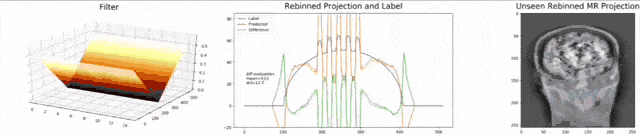
We can now also train view-dependent filters. So, this is what you see here. Now, we have a filter for every different view that is acquired. We can still show the difference between the predicted image and the label image and again directly applied to our anthropomorphic phantom. You see also in this case, we get a very good convergence. We train filters and those filters can be united in order to produce very good images of our phantom.
现在,我们还可以训练与视图相关的过滤器。 所以,这就是您在这里看到的。 现在,我们为获取的每个不同视图提供了一个过滤器。 我们仍然可以显示预测图像和标签图像之间的差异,并再次将其直接应用于拟人化模型。 您还会看到在这种情况下,我们得到了很好的融合。 我们训练滤镜,并且可以将那些滤镜组合在一起,以产生幻影的非常好的图像。
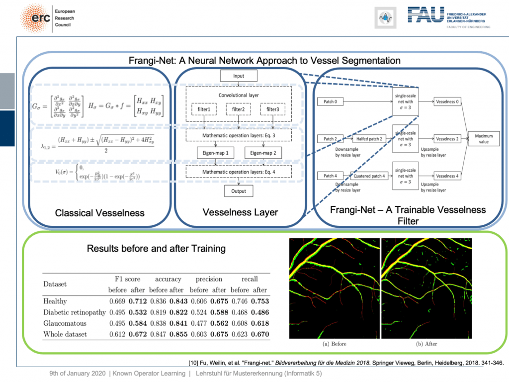
Very well, there are also other things that we can use as a kind of prior knowledge. Here is a work where we essentially took a heuristic method, the so-called vesselness filter that has been proposed by Frangi. You can show that the processing that it does is essentially convolutions. There’s an eigenvalue computation. But if you look at the eigenvalue computation, you can see that this central equation here. It can also be expressed as a layer and this way we can map the entire computations of the Frangi filter into a specialized kind of layer. This can then be trained in a multiscale approach and gives you a trainable version of the Frangi filter. Now, if you do so, you can produce vessel segmentations and they are essentially inspired by the Frangi filter but because they are trainable they produce much better results.
很好,还有其他东西可以用作先验知识。 这是我们基本上采用启发式方法的工作,这是Frangi提出的所谓的脉管滤波器。 您可以证明它所做的处理本质上是卷积。 有一个特征值计算。 但是,如果查看特征值计算,则可以在此处看到该中心方程。 它也可以表示为一层,这样我们就可以将Frangi过滤器的整个计算映射到一种特殊的层中。 然后可以采用多尺度方法对其进行训练,并为您提供Frangi过滤器的可训练版本。 现在,如果您这样做,就可以进行血管分割,并且它们实质上是受Frangi过滤器启发的,但是由于它们是可训练的,因此可以产生更好的结果。
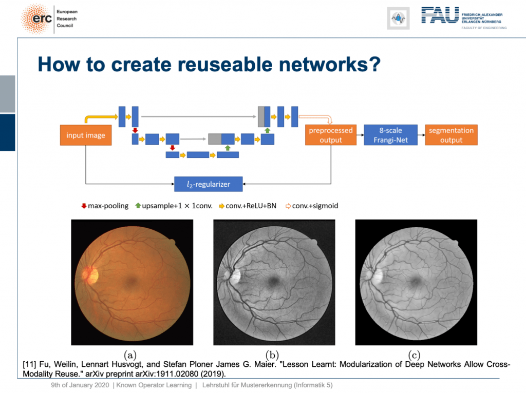
This is kind of interesting, but you very quickly realize that one reason why the Frangi filter fails is inadequate pre-processing. So, we can also combine this with a kind of pre-processing network. Here, the idea then is that you take let’s say a U-net or a guided filter network. Also, the guided filter or by the way the joint bilateral filter can be mapped into neural network layers. You can include them here and you design a special loss. This special loss is not just optimizing the segmentation output, but you combine it with some kind of autoencoder loss here. So in this layer, you want to have a pre-processed image that is still similar to the input, but with properties such that the vessel segmentation using an 8 scale Frankie filter is much better. So, we can put this into our network and train it. As a result, we get vessel detection and this vessel detection is on par with a U-net. Now, the U-Net is essentially a black box method, but here we can say “Okay, we have a kind of pre-processing net.” By the way, using a guided filter, it works really well. So, it doesn’t have to be a U-net. This is kind of a neural network debugging approach. You can show that we can now module by module replace parts of our U-net. In the last version, we don’t have U-nets at all anymore, but we have a guided filter network here and the Frangi filter. This has essentially the same performance as the U-net. So, this way we are able to modularize our networks. Why would you want to create modules? Well, the reason is modules are reusable. So here, you see the output on eye imaging data of ophthalmic data. This is a typical fundus image. So it’s an RGB image of the eye background. It shows the blind spot where the vessels all penetrate the retina. The fovea is where you have essentially the best resolution on your retina. Now, typically if you want to analyze those images, you would just take the green color Channel because it’s the channel of the highest contrast. The result of our pre-processing network can be shown here. So, we get significant noise reduction, but at the same time, we also get this emphasis on vessels. So, it kind of improves how the vessels are displayed and also fine vessels are preserved.
这很有意思,但是您很快就会意识到Frangi过滤器失败的原因之一是预处理不足。 因此,我们也可以将其与一种预处理网络结合起来。 在这里,我们的想法是假设您使用一个U-net或一个引导过滤器网络。 而且,引导滤波器或通过联合双边滤波器可以映射到神经网络层。 您可以在此处包括它们,并且可以设计特殊的损耗。 这种特殊的损失不仅是优化分段输出,而且在这里将其与某种自动编码器损失结合在一起。 因此,在此层中,您需要一个预处理后的图像,该图像仍与输入相似,但具有的属性使得使用8比例Frankie滤波器进行血管分割要好得多。 因此,我们可以将其放入我们的网络并对其进行培训。 结果,我们得到了船只检测,并且该船只检测与U-net相当。 现在,U-Net本质上是一种黑匣子方法,但是在这里我们可以说“好的,我们有一种预处理网络。” 顺便说一句,使用导向滤镜,它确实运行良好。 因此,它不必是U-net。 这是一种神经网络调试方法。 您可以证明我们现在可以逐模块更换U-net的各个部分。 在最后一个版本中,我们再也没有U-net了,但是这里有一个引导过滤器网络和Frangi过滤器。 这与U-net具有基本相同的性能。 因此,通过这种方式,我们可以使我们的网络模块化。 您为什么要创建模块? 好吧,原因是模块是可重用的。 因此,在这里,您将看到眼科数据在眼部成像数据上的输出。 这是典型的眼底图像。 这是眼睛背景的RGB图像。 它显示了血管全部穿透视网膜的盲点。 中央凹是视网膜上分辨率最高的地方。 现在,通常,如果您要分析这些图像,则只需选择绿色通道,因为它是对比度最高的通道。 我们的预处理网络的结果可以在此处显示。 因此,我们获得了显着的降噪效果,但与此同时,我们也将重点放在了船只上。 因此,它改善了容器的展示方式,并保留了精美的容器。
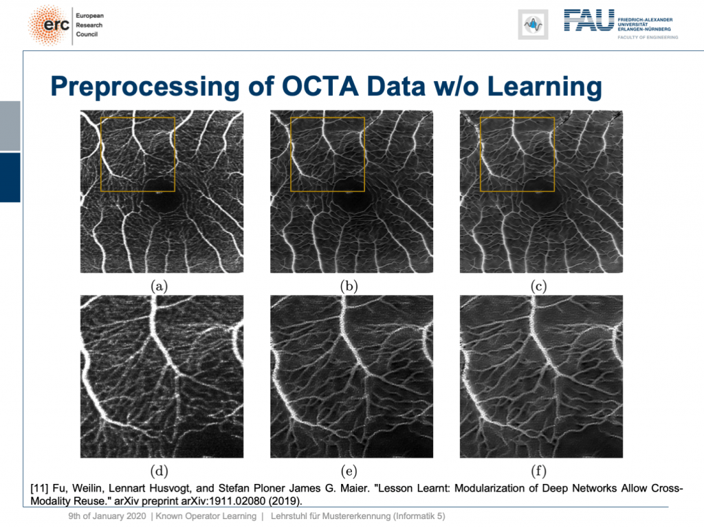
Okay, this is nice, but it only works on fundus data, right? No, our modularization shows that if we take this kind of modeling, we are able to transfer the filter to a completely different modality. This is now optical cohere tomography angiography (OCTA), a specialist modality in order to extract contrast-free vessel images of the eye background. You can now demonstrate that our pre-processing filter can be applied to these data without any additional need for fine-tuning, learning, or whatnot. You take this filter and apply it to the en-face images that, of course, show similar anatomy. But you don’t need any training on OCTA data at all. This is the OCTA input image on the left. This is the output of our filter, in the center, and this is a 50% blend of the two, on the right. Here, we have the magnified areas and you can see very nicely that what is appearing like noise is actually reformed into vessels in the output of our filter. Now, these are qualitative results. By the way, until now we finally also have quantitative results and we are actually quite happy that our pre-processing network is really able to produce the vessels at the right locations. So, this is a very interesting result and this shows us that we kind of can modularize networks and make them reusable without having to train them. So, we can now probably generate blocks that can be reassembled to new networks without additional adjustment and fine-tuning. This is actually pretty cool.
好的,这很好,但是仅适用于眼底数据,对吧? 不,我们的模块化表明,如果我们采用这种建模,我们就能将过滤器转移到完全不同的模态。 现在这是光学相干断层扫描血管造影(OCTA),这是一种专业模式,用于提取眼睛背景的无对比度血管图像。 现在,您可以证明我们的预处理过滤器可以应用于这些数据,而无需进行任何其他微调,学习或其他操作。 您可以使用此滤镜并将其应用于当然显示出类似解剖结构的面部图像。 但是您根本不需要任何有关OCTA数据的培训。 这是左侧的OCTA输入图像。 这是我们过滤器的输出,位于中间,这是两者的50%混合,位于右侧。 在这里,我们有放大的区域,您可以非常清楚地看到,实际上出现的噪声实际上已在滤波器的输出中重新形成为血管。 现在,这些是定性结果。 顺便说一句,到目前为止,我们最终也获得了定量的结果,我们对我们的预处理网络确实能够在正确的位置生产船只感到非常满意。 因此,这是一个非常有趣的结果,它向我们表明,我们可以对网络进行模块化,并使它们可重用,而无需进行培训。 因此,我们现在可以生成无需重新调整和微调即可重新组装到新网络的块。 这实际上很酷。
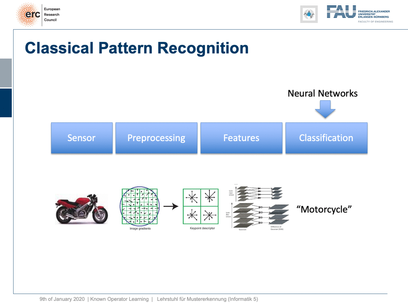
Well, this essentially leads us back to our classical pattern recognition pipeline. You remember, we looked at that in the very beginning. We have the sensor, the pre-processing, the features, and the classification. The classical role of neural networks was just classifying and you had all these feature engineering on the path here. We said that’s much better to do deep learning because then we do everything end-to-end and we can optimize all on the way. Now, if we look at this graph then we can also think about whether we actually need something like neural network design patterns. One design pattern is of course the end-to-end learning, but you may also want to include these autoencoder pre-processing losses in order to get the maximum out of your signals. On the one hand, you want to make sure that you have an interpretable module here that still remains in the image domain. On the other hand, you want to have good features and another thing that we learned about in this class is multi-task learning. So, multi-task learning associates the same latent space with different problems with different classification results. This way by implementing a multi-task loss, we make sure that we get very general features and features that will be applicable to a wide range of different tasks. So, essentially we can see that by appropriate construction of our loss functions, we’re actually back to our classical pattern recognition pipeline. It’s not the same pattern recognition pipeline that we had in a classical sense because everything is end-to-end and differentiable. So, you could argue that what we’re going towards right now is CNNs, ResNets, global pooling, differentiable rendering even are kinds of known operations that are embedded into those networks. We then essentially get modules that can be recombined and we probably end up in differentiable algorithms. This is the path that we’re going: Differentiable, adjustable algorithms that can be fine-tuned using only a little bit of data.
好吧,这实质上使我们回到了传统的模式识别管道。 您还记得,我们从一开始就看过它。 我们有传感器,预处理,功能和分类。 神经网络的经典作用只是分类,在这里的路径上已经有了所有这些特征工程。 我们说深度学习要好得多,因为那样我们就可以端到端地做所有事情,并且可以一路优化。 现在,如果我们看一下这张图,我们还可以考虑我们是否真的需要诸如神经网络设计模式之类的东西。 一种设计模式当然是端到端学习,但是您可能还希望包括这些自动编码器的预处理损耗,以便最大程度地利用信号。 一方面,您要确保此处有一个可解释的模块,该模块仍保留在映像域中。 另一方面,您希望具有良好的功能,而在本课程中我们学到的另一件事是多任务学习。 因此,多任务学习将相同的潜在空间与不同的问题与不同的分类结果相关联。 这样,通过实现多任务丢失,我们确保获得非常通用的功能,并将这些功能应用于各种不同的任务。 因此,从本质上我们可以看到,通过适当构建损失函数,我们实际上又回到了传统的模式识别管道。 这与传统意义上的模式识别流水线不同,因为一切都是端到端且可区分的。 因此,您可能会争辩说,我们现在要使用的是CNN,ResNets,全局池,可区分的呈现,甚至是嵌入到这些网络中的已知操作。 然后,我们实质上获得了可以重组的模块,并且最终可能会得出可区分的算法。 这就是我们要走的路:可微调的可调算法,仅需少量数据即可对其进行微调。
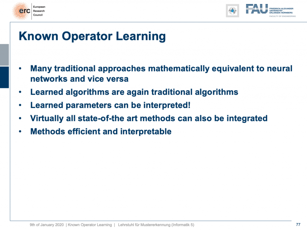
I wanted to show to you this concept because I think known operator learning is pretty cool. It also means that you don’t have to throw away all of the classical theory that you already learned about: Fourier transforms and all the clever ways of how you can process a signal. They still are very useful and they can be embedded into your networks, not just using regularization and losses. We’ve already seen when we talked about this bias-variance tradeoff, this is essentially one way how you can reduce variance and bias at the same time: You incorporate prior knowledge on the problem. So, this is pretty cool. Then, you can create algorithms, learn the weights, you reduce the number of parameters. Now, we have a nice theory that also shows us that what we are doing here is sound and virtually all of the state-of-the-art methods can be integrated. There are very few operations where you cannot find a subgradient approximation. If you don’t find a subgradient approximation, there are probably also other ways around it, such that you can still work with it. This makes methods very efficient, interpretable, and you can also work with modules. So, that’s pretty cool, isn’t it?
我想向您展示这个概念,因为我认为已知的操作员学习非常酷。 这也意味着您不必抛弃已经学到的所有经典理论:傅里叶变换以及如何处理信号的所有巧妙方法。 它们仍然非常有用,可以嵌入到您的网络中,而不仅仅是使用正则化和丢失。 当我们谈论偏差-偏差权衡时,我们已经看到了,这实质上是您可以同时减少偏差和偏差的一种方式:您将有关问题的先验知识纳入其中。 因此,这非常酷。 然后,您可以创建算法,学习权重,减少参数数量。 现在,我们有了一个很好的理论,这也向我们表明,我们在这里所做的一切都是合理的,并且几乎所有最新技术都可以集成。 很少有操作无法找到次梯度近似值。 如果找不到次梯度近似值,则可能还有其他解决方法,因此您仍然可以使用它。 这使方法非常有效,易于解释,并且您也可以使用模块。 所以,这很酷,不是吗?
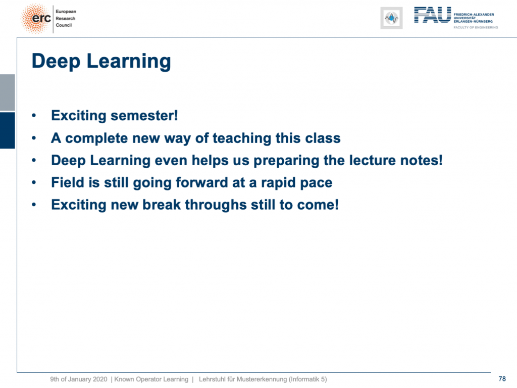
Well, this is our last video. So, I also want to thank you for this exciting semester. This is the first time that I am entirely teaching this class in a video format. So far, what I heard, the feedback was generally very positive. So, thank you very much for providing feedback on the way. This is also very crucial and you can see that we improved on the lecture on various occasions in terms of hardware and also in what to include, and so on. Thank you very much for this. I had a lot of fun with this and I think a lot of things I will also keep on doing in the future. So, I think these video lectures are a pretty cool way, in particular, if you’re teaching a large class. In the non-corona case, this class would have an audience of 300 people and I think, if we use things like these recordings, we can also get a very personal way of communicating. I can also use the time that I don’t spend in the lecture hall for setting up things like question and answer sessions. So, this is pretty cool. The other thing that’s cool is we can even do lecture notes. Many of you have been complaining, the class doesn’t have lecture notes and I said “Look, we make this class up-to-date. We include the newest and coolest topics. It’s very hard to produce lecture notes.” But actually, deep learning helps us to produce lecture notes because have video recordings. We can use speech recognition on the audio track and produce lecture notes. So you see that I already started doing this and if you go back to the old recordings, you can see that I already put in links to the full transcript. They’re published as blog posts and you can also access them. By the way, like the videos are the blog posts and everything that you see here licensed using Creative Commons BY 4.0 which means you are free to reuse any part of this and redistribute and share it. So generally, I think this field of machine learning and in particular, deep learning methods we’re going at a rapid pace right now. We are still going ahead. So, I don’t see that these things and developments will stop very soon and there’s still very much excitement in the field. I’m also very excited that I can show the newest things to you in lectures like this one. So, I think there are still exciting new breakthroughs to come and this means that we will adjust this lecture also in the future, produce new lecture videos in order to be able to incorporate the newest latest and greatest methods.
好,这是我们的最后一个视频。 所以,我也要感谢你这个令人兴奋的学期。 这是我第一次完全以视频格式授课。 到目前为止,据我所知,反馈总体上是非常积极的。 因此,非常感谢您提供有关此方法的反馈。 这也是非常关键的,您可以看到我们在各种场合的讲座中对硬件,包含的内容等进行了改进。 非常感谢你。 我对此很开心,我认为将来我还会继续做很多事情。 因此,我认为这些视频讲座是一种非常酷的方式,特别是如果您要教授大型课程。 在非电晕的情况下,该班级将有300名观众,我想,如果我们使用这些录音之类的东西,我们也会获得非常个人化的沟通方式。 我还可以将闲暇时间用于安排问答会议等活动。 因此,这非常酷。 另一个很酷的事情是,我们甚至可以做笔记。 你们中的许多人一直在抱怨,这堂课没有讲义,我说:“看,我们使这堂课是最新的。 我们包括最新和最酷的主题。 编写讲义非常困难。” 但是实际上,深度学习可以帮助我们产生备忘录,因为它们具有视频录制功能。 我们可以在音轨上使用语音识别并生成讲义。 因此,您看到我已经开始执行此操作,并且如果您返回到旧唱片,则可以看到我已经插入了完整成绩单的链接。 它们以博客文章的形式发布,您也可以访问它们。 顺便说一句,就像视频一样,这些都是博客文章,并且您在此处看到的所有内容都使用Creative Commons BY 4.0进行了许可,这意味着您可以自由地重用其中的任何部分,然后重新分发和共享。 因此,总的来说,我认为我们现在正在快速发展这一机器学习领域,尤其是深度学习方法。 我们仍在继续。 因此,我认为这些事情和发展不会很快停止,并且该领域仍然会充满兴奋。 我很高兴能在这样的演讲中向您展示最新的事物。 因此,我认为仍然会有激动人心的新突破,这意味着我们将来也将调整此讲座,制作新的讲座视频,以便能够采用最新的最新方法。
By the way, the stuff that I’ve been showing you in this lecture is of course not just by our group. We incorporated many, many different results by other groups worldwide and of course with results that we produced in Erlangen, we do not alone, but we are working in a large network of international partners. I think this is the way how science needs to be conducted, also now and in the future. I have some additional references. Okay. So, that’s it for this semester. Thank you very much for listening to all of these videos. I hope you had quite some fun with them. Well, let’s see I’m pretty sure I’ll teach a class next semester again. So, if you like this one, you may want to join one of our other classes in the future. Thank you very much and goodbye!
顺便说一句,我在本讲座中向您展示的内容当然不仅限于我们小组。 我们并入了世界各地其他小组的许多不同结果,当然还有我们在埃尔兰根(Erlangen)产生的结果,我们并不孤单,但我们正在一个庞大的国际合作伙伴网络中工作。 我认为这是现在和将来都需要进行科学的方式。 我还有一些其他参考。 好的。 所以,这是本学期。 非常感谢您收听所有这些视频。 希望您和他们玩得很开心。 好吧,让我们看看我很确定我会在下个学期再次教一门课。 因此,如果您喜欢这个课程,将来可能想加入我们的其他课程之一。 非常感谢,再见!
If you liked this post, you can find more essays here, more educational material on Machine Learning here, or have a look at our Deep LearningLecture. I would also appreciate a follow on YouTube, Twitter, Facebook, or LinkedIn in case you want to be informed about more essays, videos, and research in the future. This article is released under the Creative Commons 4.0 Attribution License and can be reprinted and modified if referenced. If you are interested in generating transcripts from video lectures try AutoBlog.
如果你喜欢这篇文章,你可以找到这里更多的文章 ,更多的教育材料,机器学习在这里 ,或看看我们的深入 学习 讲座 。 如果您希望将来了解更多文章,视频和研究信息,也欢迎关注YouTube , Twitter , Facebook或LinkedIn 。 本文是根据知识共享4.0署名许可发布的 ,如果引用,可以重新打印和修改。 如果您对从视频讲座中生成成绩单感兴趣,请尝试使用AutoBlog 。
谢谢 (Thanks)
Many thanks to Weilin Fu, Florin Ghesu, Yixing Huang Christopher Syben, Marc Aubreville, and Tobias Würfl for their support in creating these slides.
非常感谢傅伟林,弗洛林·格苏,黄宜兴Christopher Syben,马克·奥布雷维尔和托比亚斯·伍尔夫(TobiasWürfl)为创建这些幻灯片提供的支持。
翻译自: https://towardsdatascience.com/known-operator-learning-part-4-823e7a96cf5b
已知两点坐标拾取怎么操作


 被折叠的 条评论
为什么被折叠?
被折叠的 条评论
为什么被折叠?
 到【灌水乐园】发言


