怎么评价两组数据是否接近_接近组数据（组间）

怎么评价两组数据是否接近

接近组数据(组间) (Approaching group data (between-group))

A typical situation regarding solving an experimental question using a data-driven approach involves several groups that differ in (hopefully) one, sometimes more variables.

使用数据驱动的方法解决实验性问题的典型情况涉及几个组(希望)不同，有时甚至更多。

Say you collect data on people that either ate (Group 1) or did not eat chocolate (Group 2). Because you know the literature very well, and you are an expert in your field, you believe that people that ate chocolate are more likely to ride camels than people that did not eat the chocolate.

假设您收集的是吃过(第1组)或没有吃巧克力(第2组)的人的数据。 因为您非常了解文献，并且您是该领域的专家，所以您认为吃巧克力的人比没有吃巧克力的人骑骆驼的可能性更高。

You now want to prove that empirically.

您现在想凭经验证明这一点。

I will be generating simulation data using Python, to demonstrate how permutation testing can be a great tool to detect within group variations that could reveal peculiar patterns of some individuals. If your two groups are statistically different, then you might explore what underlying parameters could account for this difference. If your two groups are not different, you might want to explore whether some data points still behave “weirdly”, to decide whether to keep on collecting data or dropping the topic.

我将使用Python生成仿真数据，以演示置换测试如何成为检测组内变异的好工具，这些变异可以揭示某些个体的特殊模式。 如果两组在统计上不同，那么您可能会探索哪些基础参数可以解释这一差异。 如果两组没有不同，则可能要探索某些数据点是否仍然表现“怪异”，以决定是继续收集数据还是删除主题。

# Load standard libraries
import panda as pd 
import numpy as np
import matplotlib.pyplot as plt

Now one typical approach in this (a bit crazy) experimental situation would be to look at the difference in camel riding propensity in each group. You could compute the proportions of camel riding actions, or the time spent on a camel, or any other dependent variable that might capture the effect you believe to be true.

现在，在这种(有点疯狂)实验情况下，一种典型的方法是查看每组中骑骆驼倾向的差异。 您可以计算骑骆驼动作的比例，骑骆驼的时间或其他任何可能捕捉到您认为是真实的效果的因变量。

产生资料 (Generating data)

Let’s generate the distribution of the chocolate group:

让我们生成巧克力组的分布：

# Set seed for replicability
np.random.seed(42)# Set Mean, SD and sample size
mean = 10; sd=1; sample_size=1000# Generate distribution according to parameters
chocolate_distibution = np.random.normal(loc=mean, scale=sd, s
size=sample_size)# Show data
plt.hist(chocolate_distibution)
plt.ylabel("Time spent on a camel")
plt.title("Chocolate Group")

As you can see, I created a distribution centered around 10mn. Now let’s create the second distribution, which could be the control, centered at 9mn.

如您所见，我创建了一个以1000万为中心的发行版。 现在，让我们创建第二个分布，该分布可能是控件，以900万为中心。

mean = 9; sd=1; sample_size=1000
non_chocolate_distibution = np.random.normal(loc=mean, scale=sd, size=sample_size)
fig = plt.figure()
plt.hist(non_chocolate_distibution)
plt.ylabel("Time spent on a camel")
plt.title("Non Chocolate Group")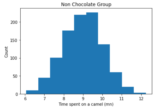

Figure 2 | Histogram depicting the number of people that rode the camel in the Non Chocolate group, splited per minutes bin.

图2 | 直方图描述了非巧克力组中骑骆驼的人数，每分钟垃圾箱划分的人数。

OK! So now we have our two simulated distributions, and we made sure that they differed in their mean. With the sample size we used, we can be quite sure we would have two significantly different populations here, but let’s make sure of that. Let’s quickly visualize that:

好！ 因此，现在我们有了两个模拟分布，并确保它们的均值不同。 使用我们使用的样本量，我们可以确定这里会有两个明显不同的总体，但是让我们确定一下。 让我们快速想象一下：

Figure 3 | Both chocolate and non chocolate distributions seen together.

图3 | 可以同时看到巧克力和非巧克力的分布。

We can use an independent sample t-test to get an idea of how different these distributions might be. Note that since the distributions are normally distributed (you can test that with a Shapiro or KS test), and the sample size is very high, parametric testing (under which t-test falls) is permitted. We should run a Levene’s test as well to check the homogeneity of variances, but for the sake of argumentation, let’s move on.

我们可以使用独立的样本t检验来了解这些分布可能有多大差异。 请注意，由于分布是正态分布的(可以使用Shapiro或KS检验进行测试)，并且样本量非常大，因此可以进行参数检验(t检验属于这种检验)。 我们也应该运行Levene检验来检验方差的均匀性，但是为了论证，让我们继续。

from scipy import stats
t, p = stats.ttest_ind(a=chocolate_distibution, b=non_chocolate_distibution, axis=0, equal_var=True)
print('t-value = ' + str(t))
print('p-value = ' + str(p))

Output of an independent sample t test between the two distributions.

两个分布之间的独立样本t检验的输出。

Good, that worked as expected. Note that given the sample size, you are able to detect eve