fifa11键盘按键_FIFA 20 Player集群

fifa11键盘按键

路线图 (Roadmap)

• Introduction

  介绍

• Data Exploration

  数据探索

• Player Classification1 — K-Nearest Neighbor

  玩家分类1 — K最近邻居

  Player Classification1 — K-Nearest Neighbor2 — Decision Tree Classifier

  玩家分类1 — K最近邻居2 — 决策树分类器

  Player Classification1 — K-Nearest Neighbor2 — Decision Tree Classifier3 — Support Vector Machine

  玩家分类1 — K最近邻居2 — 决策树分类器3 — 支持向量机

  Player Classification1 — K-Nearest Neighbor2 — Decision Tree Classifier3 — Support Vector Machine4 — Logistic Regression

  玩家分类1 — K最近邻居2 — 决策树分类器3 — 支持向量机4 — 逻辑回归

• Results

  结果

• Conclusions

  结论

介绍 (Introduction)

FIFA is a football simulation game, released each year by Electronic Arts Inc, the main characters of the video game, of course, the football players. Players on the video game are intended to be as close as the real ones, both physically and in skills. This set of skills determine the position they play on the field. Of course, you want a killer striker and a wall as a goalkeeper!

FIFA是一款足球模拟游戏，由电子艺术公司每年发行，这是视频游戏的主要角色，当然还有足球运动员。 电子游戏的玩家无论在身体上还是技能上都应与真实玩家尽可能接近。 这套技能决定了他们在球场上的位置。 当然，您想要杀手级的前锋和一堵墙作为守门员！

目的 (Objective)

If you are a football fan, you most likely know the position each player has on your favorite team. Can a machine learn the different player’s position according to their skills?

如果您是足球迷，那么您很可能知道每个球员在您喜欢的球队中所处的位置。 机器可以根据他们的技能来学习其他玩家的位置吗？

获取数据 (Obtaining the data)

Data was downloaded from Kaggle, which was scraped from the publicly available website sofifa.

数据是从Kaggle下载的，该数据是从可公开获取的网站sofifa上抓取的 。

数据探索 (Data Exploration)

The first step is to download the data and take a first look at some of the information of the players.

第一步是下载数据并首先查看播放器的一些信息。

Now let’s take a look at the players that will make a club pay “top dollar”.

现在，让我们看一下将使俱乐部支付“最高价”的球员。

演示地址

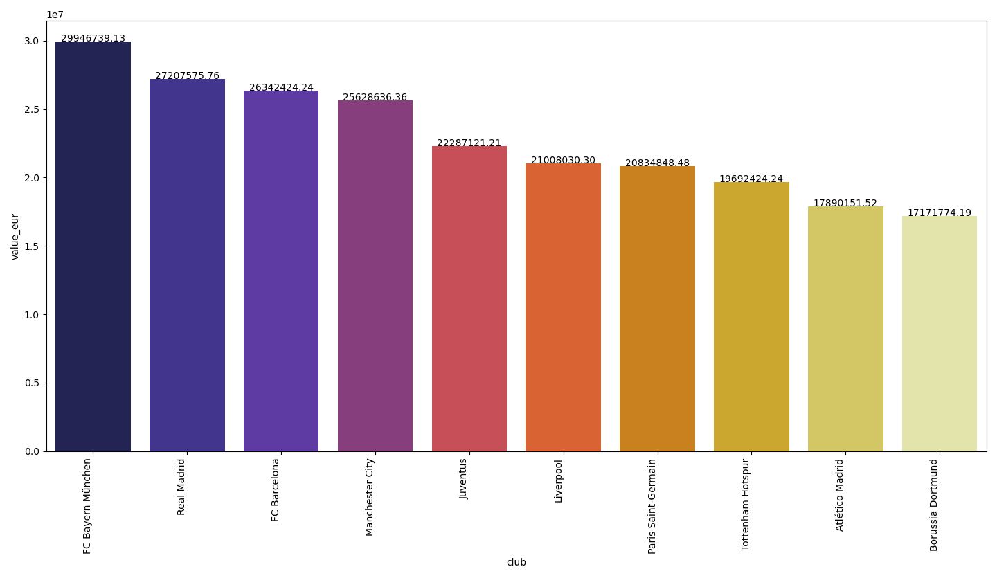
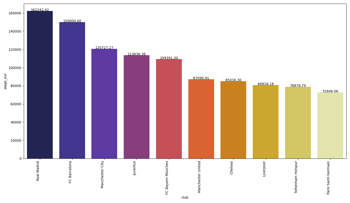
These two players are definitely expensive, but which clubs spend on average the most? In order to show this, players where grouped by club, then the mean was taken from columns “value_eur” and “wage_eur”.

这两个球员肯定是昂贵的，但是哪个俱乐部平均花费最多？ 为了显示这一点，将球员按俱乐部分组，然后从“ value_eur”和“ wage_eur”列中取平均值。

Let’s take a look at the top 10 clubs with the most valuable players and top 10 clubs which pay the highest wages.

让我们看一下拥有最有价值球员的前十名俱乐部和支付最高工资的前十名俱乐部。

Average player value (for reference, first value is 29.9 million euros)

平均球员价值(作为参考，第一价值为2990万欧元)

Average wage paid to player (fore reference, first value is 162.2 thousand euros)

支付给玩家的平均工资(参考之前，第一价值为16.22万欧元)

Now let’s have a look at the clubs with the top players.

现在，让我们来看看拥有顶级球员的俱乐部。

Average players overall

总体平均水平

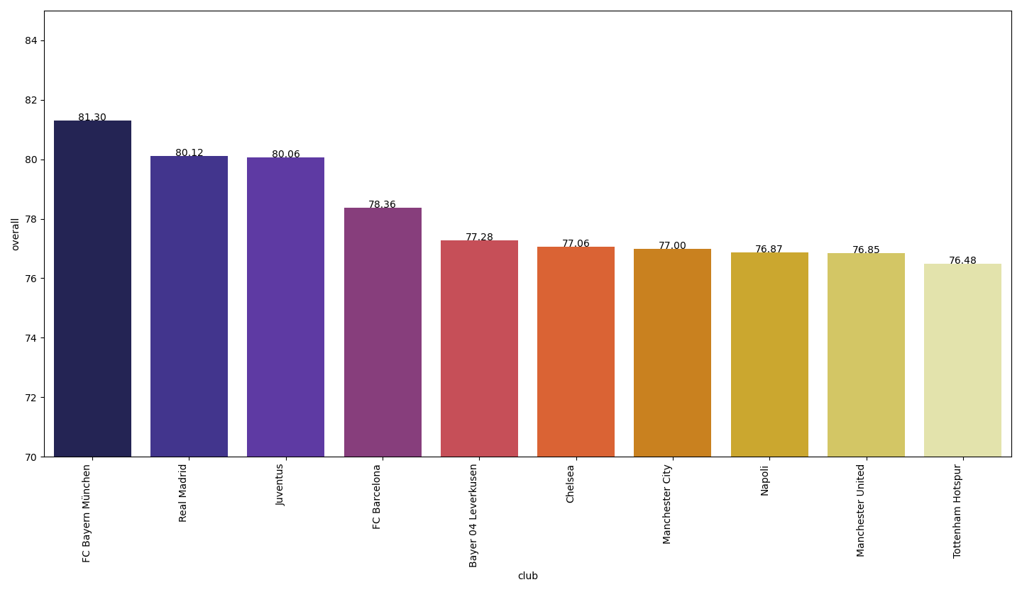
Note: This doesn’t necessarily translate into a plot of best teams, since some clubs may have more substitute or reserve players than others, nonetheless, an interesting output.

注意：这不一定会转化为最佳球队，因为尽管如此，有些俱乐部可能拥有比其他俱乐部更多的替补或替补球员，这是一个有趣的输出。

The country with more leagues on FIFA 20 is England, no surprise they have the most number of players in the game.

在FIFA 20联赛中排名最高的国家是英格兰，毫不奇怪，他们在比赛中拥有最多的球员。

演示地址

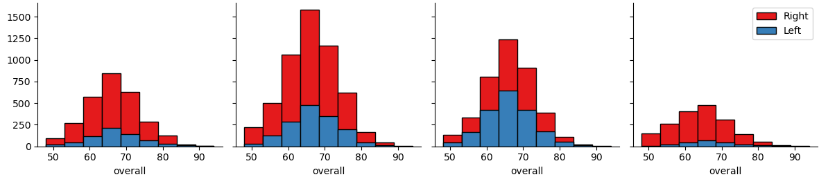
The histograms below show some interesting insights:

下面的直方图显示了一些有趣的见解：

• The majority of players are right-footed.
  大多数球员都是右脚。
• Left tail cuts sharply at around an overall of 50 (considering these are players at a professional team it shouldn’t go longer to the left, right?).
  左尾锋锐利地砍下了大约50杆(考虑到这些是专业团队的球员，它不应该向左走更长的时间，对吗？)。
• Right tail is long and represents a minority of exceptional players.
  右尾很长，代表少数优秀球员。
• Center of the field is “busier” than the ends, there are more midfielders and defenders than strikers and goalkeepers.
  领域的中心比目标更“忙”，中场和后卫比前锋和守门员更多。

From left to right: Attackers, Midfielders, Defenders and Goalkeepers

从左至右：攻击者，中场，后卫和守门员

Histograms above are divided by player positions, we can take a look at the general distribution of the “Overall” score.

上面的直方图按玩家位置划分，我们可以看看“总体”得分的总体分布。

演示地址

数据预处理 (Data Preprocessing)

球员位置 (Player positions)

If we take a look at player positions, we notice players have one position, others have two and some even three!

如果我们看一下玩家的位置，就会发现玩家有一个位置，其他有两个，甚至三个！

演示地址

For the scope of this project, positions will be grouped in four categories

对于该项目的范围，职位将分为四个类别

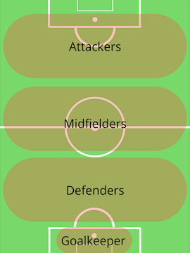
• Attackers: ST, LW, RW, CF
  攻击者：ST，LW，RW，CF
• Midfielders: CAM, LM, CM, RM, CDM
  中场：CAM，LM，CM，RM，CDM
• Defenders: LWB, RWB, LB, CB, RB
  防御者：LWB，RWB，LB，CB，RB
• Goalkeepers: GK
  守门员：GK

Correctly grouping players in these categories is an important step before making any model. Let’s take for example the player “41”, this player has three positions:

在制作任何模型之前，将这些类别的玩家正确分组是重要的一步。 让我们以玩家“ 41”为例，该玩家具有三个位置：

• RW — Attacker
  RW-攻击者
• CAM — Midfielder
  CAM —中场
• CM — Midfielder
  CM —中场

If we select just the first position for each player, this “41” player would be considered as an “Attacker”, however, he also plays in two other positions, both as a “Midfielder”. So a better approach would be to consider this player a midfielder. To make this possible the following function was created and applied to the ‘player_positions’ column.

如果我们仅为每个玩家选择第一个位置，则该“ 41”玩家将被视为“攻击者”，但是，他还在另外两个位置中都扮演“中场手”。 因此，更好的方法是将这位球员视为中场球员。 为了使之成为可能，创建了以下函数并将其应用于“ player_positions”列。

演示地址

分割数据 (Splitting the data)

A new DataFrame is created which will have only the useful columns, these are shown below with the number of null values.

创建一个新的DataFrame，它仅包含有用的列，这些列如下所示，其中包含空值的数量。

演示地址

We have 0 null values in our DataFrame so we can proceed.

我们的DataFrame中有0个空值，因此我们可以继续进行。

The data values will be assigned accordingly, predictors (X) and target (y), then it will be split into train and test.

数据值将相应地分配，预测变量(X)和目标变量(y)，然后将其分为训练和测试。

• X will include all skills from players.
  X将包括玩家的所有技能。
• y will include player position.
  y将包括玩家位置。

Inputs from train_test_split:

来自train_test_split的输入：

• test_size=0.2 — Train data will be 80% and test will be 20%.
  test_size = 0.2-火车数据将为80％，测试数据将为20％。
• random_state=42 — Used to seed a new RandomState object.
  random_state = 42 —用于播种新的RandomState对象。
• stratify=y — Makes the values splitted proportional.
  stratify = y —使值按比例分割。

演示地址

Although the standardization of the data is an important pre-process, this will be executed in combination with each machine learning model and cross-validation through Pipeline to avoid leakage.

尽管数据的标准化是一个重要的预处理过程，但这将与每种机器学习模型和通过管道进行的交叉验证结合起来执行，以避免泄漏。

So what are these terms? Here is a brief explanation of each:

那么这些术语是什么呢？ 这是每个的简要说明：

资料外泄 (Data leakage)

When information from outside the training dataset is used to create the model.

当使用来自训练数据集外部的信息来创建模型时。

标准化 (Standardization)

Data standardization is the process of rescaling one or more attributes so that they have a mean value of 0 and a standard deviation of 1.

数据标准化是重新缩放一个或多个属性的过程，以使它们的平均值为0，标准差为1。

管道 (Pipeline)

According to scikit-learn documentation: Sequentially apply a list of transforms and a final estimator. Intermediate steps of the pipeline must be ‘transforms’, that is, they must implement fit and transform methods. The final estimator only needs to implement fit.

根据scikit-learn文档：依次应用转换列表和最终估计量。 流水线的中间步骤必须是“转换”，也就是说，它们必须实现拟合和转换方法。 最终估算器只需实现拟合。

The purpose of the pipeline is to assemble several steps that can be cross-validated together while setting different parameters.

流水线的目的是组装几个步骤，这些步骤可以在设置不同参数的同时交叉验证。

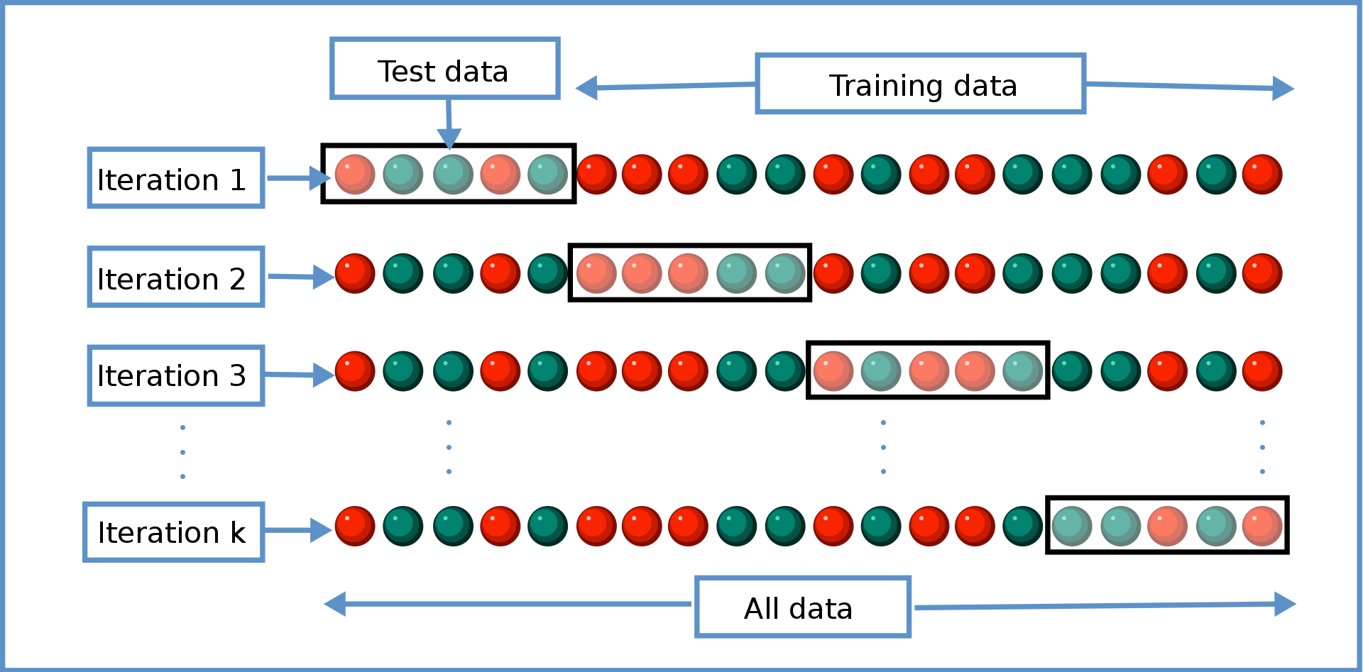
K折交叉验证 (K-fold Cross-validation)

Splitting the data into train and test is necessary for supervised learning, however, the results of the model will be based on this only partition. A solution to this problem is a procedure called k-fold cross-validation, where data is divided in k smaller sets. The training data will be k-1 folds, the remaining fold will be used for validation, average of the validation results across the k-folds will be the performance measure.

将数据分为训练和测试对于监督学习是必需的，但是，模型的结果将基于此唯一分区。 解决此问题的方法是称为k倍交叉验证的过程，该过程将数据分为k个较小的集合。 训练数据将为k-1倍，其余倍数将用于验证， k折中验证结果的平均值将作为性能指标。

This procedure could be computationally expensive, but it helps to avoid overfitting or selection bias.

此过程可能在计算上昂贵，但有助于避免过度拟合或选择偏差。

Wikipedia. 维基百科 。

球员分类 (Player Classification)

Before jumping into different machine learning models to classify players position, let’s see the correlation matrix between player attributes.

在进入不同的机器学习模型对玩家位置进行分类之前，让我们看一下玩家属性之间的相关矩阵。

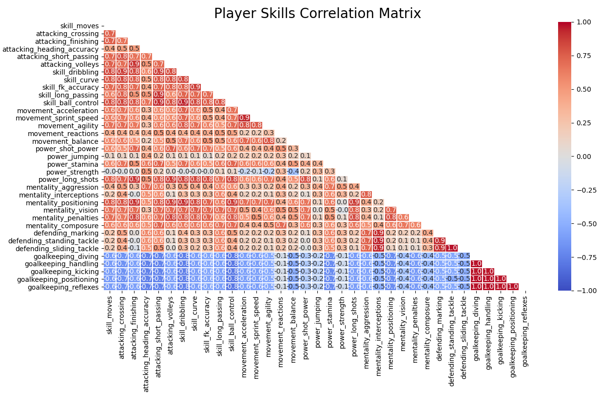
By looking at this heat map, we can assume that models should easily identify Goalkeepers, let’s find out how they perform.

通过查看此热图，我们可以假定模型应该轻松识别守门员，让我们找出他们的表现。

Note: There will be a brief explanation of each classification algorithm, a deeper approach of each is out of the scope of this story. The presented explanation should be enough to understand the displayed code.

注意：将对每种分类算法进行简要说明，每种分类算法的更深层次的方法不在本文讨论范围之内。 所提供的解释应该足以理解所显示的代码。

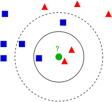
K最近邻居 (K-Nearest Neighbor)

An object is classified by a plurality vote of its neighbors, with the object being assigned to the class most common among its k nearest neighbors. If k = 1, then the object is simply assigned to the class of that single nearest neighbor.

对象通过其邻居的多次投票进行分类，该对象被分配给其k个最近邻居中最常见的类别。 如果k = 1，则仅将对象分配给该单个最近邻居的类。

The image below shows an example of how the algorithm works. The green dot is the test object. If k = 3 it will be classified as a red triangle since there are two red triangle against one blue square (circle area). If k = 5 it will now be classified as a blue square, since these “neighbors” now have the majority (dashed circle area).

下图显示了该算法如何工作的示例。 绿点是测试对象。 如果k = 3，则将其分类为红色三角形，因为相对于一个蓝色正方形(圆形区域)有两个红色三角形。 如果k = 5，则现在将其分类为蓝色正方形，因为这些“邻居”现在拥有多数(虚线圆圈区域)。

Wikipedia. 维基百科 。

The following code combines what we’ve read so far:

以下代码结合了我们到目前为止已经阅读的内容：

• Data standardization.
  数据标准化。
• Use of pipeline to link the different “pieces” (with their corresponding parameters) of the ML process.
  使用管道来链接ML过程的不同“部分”(及其相应的参数)。

• Cross-validation through the data with k-folds (k = 5) .

  通过具有k倍( k = 5)的数据进行交叉验证。

演示地址

The result is the cross-validated mean with the corresponding best parameter. Now we can fit the model and make a prediction.

结果是具有相应最佳参数的交叉验证平均值。 现在我们可以拟合模型并做出预测。

演示地址

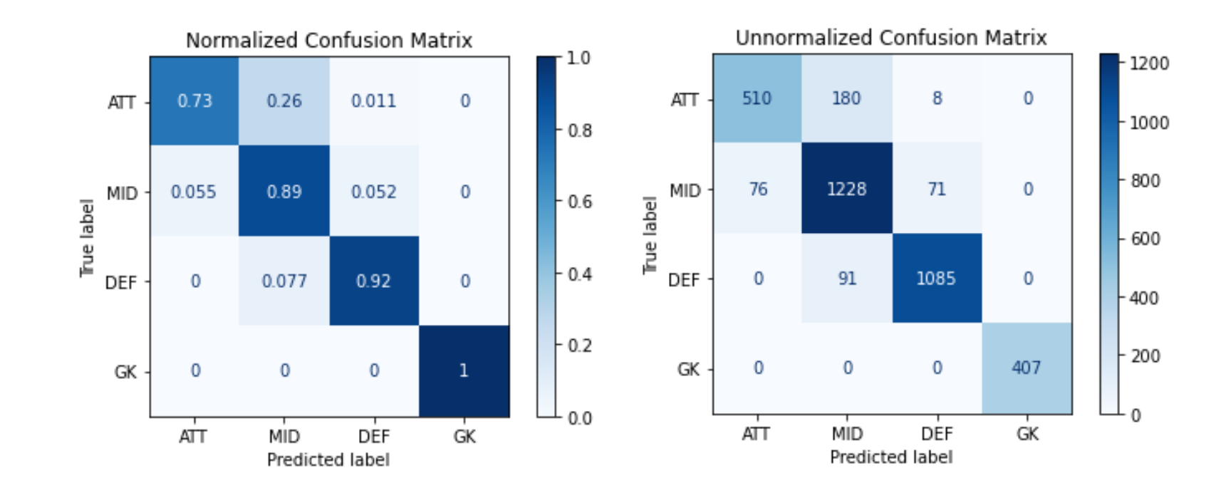
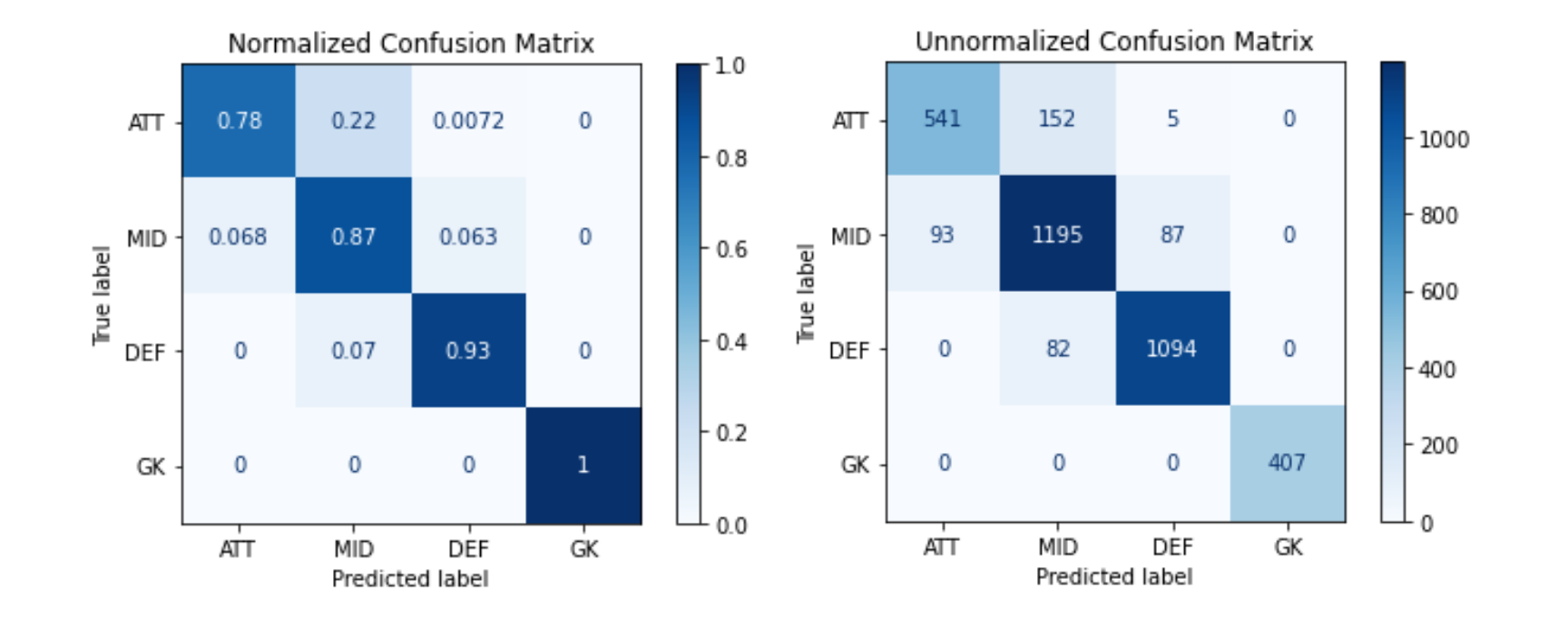
A useful tool to visualize the performance of an algorithm is the confusion matrix. This two dimension table shows the labeling of the players. The normalized shows the classification as percentage and the unnormalized as number of players. For instance:

可视化算法性能的有用工具是混淆矩阵。 二维表显示了播放器的标签。 归一化将分类显示为百分比，未归一化显示为玩家数量。 例如：

• 510 (73%) Attackers were correctly classified.
  510(73％)攻击者的分类正确。
• 180 (26%) Attackers were classified as Midfielders.
  180(26％)进攻者被列为中场。
• 8 (1.1%) Attackers were classified as Defenders.
  8(1.1％)攻击者被分类为防御者。
• 0 (0%) Attackers were classified as Goalkeepers.
  0(0％)攻击者被分类为守门员。

And so on for each position.

对于每个职位，依此类推。

K-Nearest Neighbor Confusion Matrix

K最近邻居混淆矩阵

决策树分类器 (Decision Tree Classifier)

Structure in which each internal node represents a “test” on an attribute, each branch represents the outcome of the test, and each leaf node represents a class label.

每个内部节点代表一个属性上的“测试”，每个分支代表测试的结果，每个叶节点代表一个类标签的结构。

Survival of passengers on the Titanic.

泰坦尼克号上的乘客的生存。

Composition of DTC:

DTC的组成：

• Decision Nodes: As name implies, represent a decision point of a predictor variable that will lead to the target variable.

  决策节点：顾名思义，代表将导致目标变量的预测变量的决策点。

  (example — gender)

  (例如，性别)

• Branches: Connections between nodes, represented as arrows. Each branch represents a response.

  分支：节点之间的连接，以箭头表示。 每个分支代表一个响应。

  (example — male/female)

  (例如，男性/女性)

• Leaf Nodes: Leaf nodes or terminating nodes represent the final class of the outcome.

  叶节点：叶节点或终止节点代表结果的最后一类。

  (example — died/survived)

  (示例-死亡/幸存)

Note: For our data, decision nodes will be the predictors, branches will be “≤ X” and the leaf nodes will be the player position. For example, “skill_dribbling” ≤ 55.0 → Defender.

注：对于我们的数据，决策节点将是预测，树枝将“≤X”和叶节点将是玩家的位置。 例如，“ skill_dribbling”≤55.0→后卫。

Again, we use pipeline to get the best parameters for the algorithm.

同样，我们使用管道来获得算法的最佳参数。

演示地址

Can we be sure these are the best parameters? The code below shows a demonstration on the “behind the scenes” of how the best parameters are obtained in each GridSearchCV.

我们可以确定这些是最佳参数吗？ 下面的代码演示了如何在每个GridSearchCV中获得最佳参数的“幕后”。

演示地址

As we can see, out of the 24 different possibilities, (8, 'gini') has the best score (0.858638...). Now that we have the best parameters we can fit the model.

我们可以看到，在24种不同的可能性中， (8, 'gini') (0.858638...) (8, 'gini')得分最高(0.858638...) 。 现在我们有了最好的参数，我们可以拟合模型了。

演示地址

‘gini’ is the default parameter.

“ gini”是默认参数。

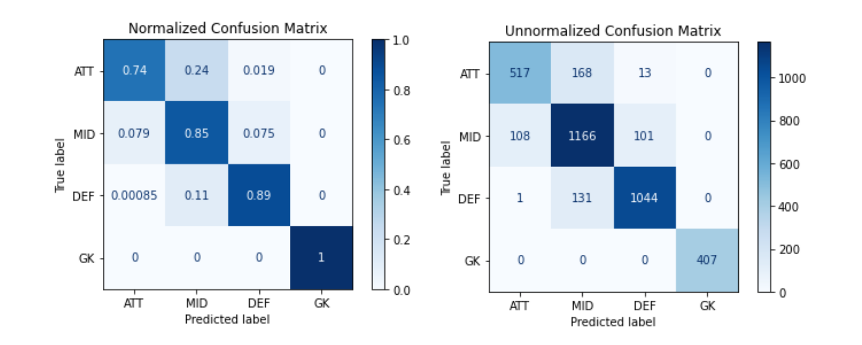
Take a look at the respective confusion matrixes.

看一下各自的混淆矩阵。

Decision Tree Classifier Confusion Matrix

决策树分类器混淆矩阵

支持向量机 (Support Vector Machine)

MathWorks. MathWorks的示例。

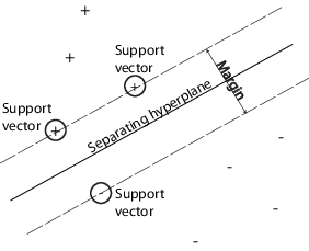
This algorithm is based on the idea of finding a hyperplane that best divides the data. The goal is to find a hyperplane with the greatest possible margin (distance) between an observation (support vector) and the hyperplane, giving a greater chance of correctly identifying new data. If the number of input features is two, then the hyperplane is just a line, if the number of input features is three, then the hyperplane becomes a two-dimensional plane. It becomes difficult to imagine when the number of features exceeds three. The idea is that the data will continue to be mapped into higher and higher dimensions until a hyperplane can be formed to segregate it.

该算法基于找到最佳分割数据的超平面的想法。 目标是找到在观测值(支持向量)和超平面之间具有最大可能余量(距离)的超平面，从而为正确识别新数据提供更大的机会。 如果输入要素的数量为两个，则超平面只是一条线，如果输入要素的数量为三个，则超平面将成为二维平面。 很难想象功能数量超过三个。 这个想法是数据将继续被映射到越来越高的维度，直到可以形成一个超平面来分离它为止。

The multi-class problem is broken down to multiple binary classification cases, which is also called one-vs-one. Which splits the dataset into one dataset for each class versus every other class.

多类问题可分解为多个二元分类案例，也称为“ 一对一” 。 它将数据集分为每个类别与每个其他类别一个数据集。

• Binary Classification Problem 1: ATT vs. MID

  二进制分类问题1 ：ATT与MID

• Binary Classification Problem 2: ATT vs. DEF

  二进制分类问题2 ：ATT与DEF

• Binary Classification Problem 3: ATT vs. GK

  二进制分类问题3 ：ATT与GK

• Binary Classification Problem 4: MID vs. DEF

  二进制分类问题4 ：MID与DEF

• Binary Classification Problem 5: MID vs. GK

  二进制分类问题5 ：MID与GK

• Binary Classification Problem 6: DEF vs. GK

  二进制分类问题6 ：DEF与GK

Each binary classification model may predict one class label and the model with the most predictions or votes is predicted by the one-vs-one strategy.

每个二元分类模型可以预测一个类别标签，并且具有最多预测或投票的模型是通过一对一策略预测的。

Note: To get a better grasp of the algorithm, notes by Andrew Ng are fantastic.

注意：为了更好地掌握算法，Andrew Ng的注释很棒。

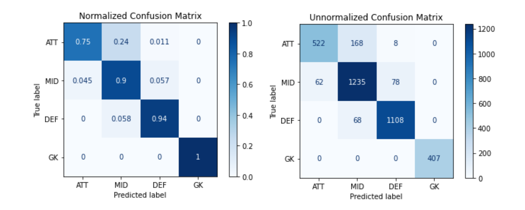
Once again, the best parameters are obtained and the model is fitted.

再次获得最佳参数并拟合模型。

演示地址

演示地址

In this case, the best parameters where the default values, so no need to type them.

在这种情况下，最好的参数位于默认值，因此无需键入它们。

Corresponding confusion matrixes.

相应的混淆矩阵。

逻辑回归 (Logistic Regression)

This model is used to predict a binary outcome given a set of features (predictors). The classifier output (target) can be 1 or 0. We are looking for the probability that an observation is part of the class (1) or not (0).

该模型用于在给定一组特征(预测变量)的情况下预测二进制结果。 分类器输出(目标)可以是1或0。我们正在寻找观察值是否属于类(1 )或不属于(0 )的可能性。

In a nutshell, it takes the features, multiplies each by a weight, sums them, and passes the sum through a sigmoid function to generate a probability and assign a class. The weights (vector w and bias b) are learned from a labeled training set via a loss function (cross-entropy loss).

简而言之，它采用特征，将每个特征乘以权重，将它们求和，然后将总和传递给S型函数以生成概率并分配类别。 权重(向量w和偏差b )是通过损失函数(交叉熵损失)从标记的训练集中学习的。

Our data has more than two targets, so we use the multinomial logistic regression which uses a generalization of the sigmoid, called the softmax function.

我们的数据有两个以上的目标，因此我们使用多项式逻辑回归，该回归使用S形的概括，称为softmax函数。

Note: Again, this is a very simplistic approach of the algorithm, find more here.

注意：同样，这是该算法的一种非常简单的方法，请在此处找到更多信息 。

Same old, same old, use pipeline to get the best parameters and fit the model.

相同，相同，使用管线来获取最佳参数并拟合模型。

演示地址

演示地址

Note: The parameter multi_class is set by default to “auto” which will select ‘“multinomial” if data isn’t binary. If “multinomial” is selected, the softmax function is used to find the predicted probability of each class to assign the target.

注意：参数multi_class默认设置为“ auto”，如果数据不是二进制的，它将选择“ multinomial”。 如果选择“多项式”，则使用softmax函数查找每个类别的预期概率以分配目标。

Last confusion matrixes.

最后的混淆矩阵。

Logistic Regression Confusion Matrix

Logistic回归混淆矩阵

结果 (Results)

As expected, all different models could easily identify Goalkeepers, the majority of skills they have seem to be negatively correlated with the rest, and strongly correlated within each other.

正如预期的那样，所有不同的模型都可以轻松地识别出守门员，他们似乎与大多数技能负相关，而彼此之间却具有很强的相关性。

We’ve seen the different confusion matrixes, let’s take a final look at some of the main classification metrics. These are obtained through classification_report and accuracy_score from the sklearn.metrics library. For simplicity, all reports are placed together in one image.

我们已经看到了不同的混淆矩阵，让我们最后看一下一些主要的分类指标。 这些都是通过获得classification_report和accuracy_score从sklearn.metrics库。 为简单起见，所有报告都放置在一个图像中。

Algorithms Classification Reports and Accuracy Score

算法分类报告和准确性得分

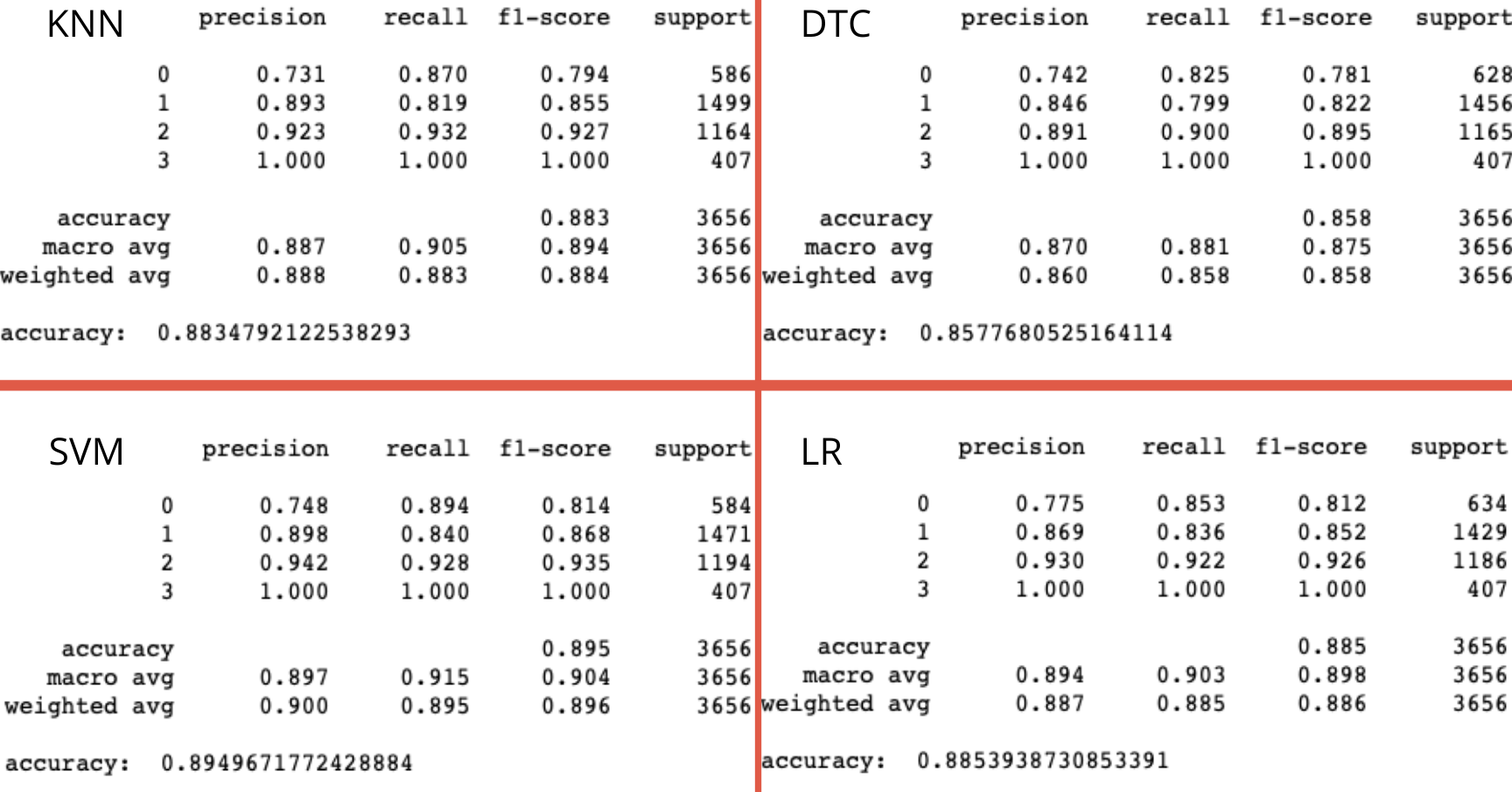
SVM seems to be the most accurate algorithm to determine players position. However, there are other important metrics. Placing an Attacker as a Defender may not be the end of the world, but certainly, it won’t perform as good. Let’s take a look at what these useful metrics bring to the table.

SVM似乎是确定玩家位置的最准确算法。 但是，还有其他重要指标。 布置进攻者作为防守者可能并非世界末日，但可以肯定的是，它的表现并不理想。 让我们看一下这些有用的指标带来了什么。

准确性 (Accuracy)

How close is the predicted value to the actual target.

预测值与实际目标有多接近。

精确 (Precision)

Fraction of relevant instances among the retrieved instances. (Diagonal values from the normalized confusion matrixes).How many selected items are relevant?

检索到的实例中相关实例的分数。 (归一化混淆矩阵的对角线值)相关的选定项目有多少？

召回 (Recall)

Fraction of the total amount of relevant instances that were actually retrieved.How many relevant items are selected?

实际检索到的相关实例总数的分数。选择了多少个相关项目？

F分数 (F-score)

Harmonic mean of precision and recall.

精确度和召回率的谐波平均值。

结论 (Conclusions)

There are several supervised algorithms, this story showed a glance at some of them. A correct pre-process of the data along with the correct selection of parameters is crucial for every algorithm.

有几种受监督的算法，这个故事对其中一些有所了解。 正确的数据预处理以及正确的参数选择对于每种算法都至关重要。

When it comes to choosing which algorithm performed better it’s important to remember:

在选择哪种算法性能更好时，请务必记住：

• Precision is a good model metric when the costs of False Positive is high.
  当误报的成本很高时，精度是一个好的模型指标。
• Recall is a good model metric when there is a high cost associated with False Negative.
  当与假阴性相关的成本很高时，召回率是一个很好的模型指标。
• F-score might be a better model metric if we need to seek a balance between precision and recall.
  如果我们需要在精度和召回率之间寻求平衡，则F评分可能是更好的模型指标。

Another important metric which sometimes is overlooked is time! Yes, you want an accurate model, but some models take more time for a small gain in accuracy. To exemplify, SVM had a 0.95% better accuracy score than Logistic Regression, however, finding the best parameters for LogReg was 6.6 times faster than SVM (both originally designed for binary classification).

有时被忽略的另一个重要指标是时间！ 是的，您需要一个准确的模型，但是某些模型花费更多的时间来获得少量的准确性。 举例来说，SVM的准确度得分比Logistic回归高0.95％，但是，发现LogReg的最佳参数比SVM快6.6倍(两者都是最初为二进制分类而设计的)。

演示地址

Time in seconds.

时间以秒为单位。

In some scenarios 1% could be a significant difference yet sometimes it may just be okay to lose that percent to get a faster result. Choosing the best algorithm depends on the attributes of your data.

在某些情况下，可能会有1％的显着差异，但有时可以丢失该百分比以获得更快的结果。 选择最佳算法取决于数据的属性。

翻译自: https://towardsdatascience.com/fifa-20-player-clustering-f500cf0792c5

fifa11键盘按键