机器学习 多变量回归算法_如何为机器学习监督算法识别正确的自变量？

机器学习 多变量回归算法

There is a very famous acronym GIGO in the field of computer science which I have learnt in my school days. GIGO stands for garbage in and garbages out. Essentially it means that if we feed inappropriate and junk data to computer programs and algorithms, then it will result in junk and incorrect results.

我在上学的时候就学过计算机科学领域的一个非常著名的缩写GIGO 。 GIGO代表垃圾进出。 从本质上讲，这意味着如果我们将不适当的垃圾数据输入计算机程序和算法，则会导致垃圾和错误结果。

Machine learning algorithms are the same as us human beings. Broadly machine learning algorithms have two phases — learning and predicting. Learning environment and parameters should be similar to the condition in which prediction to be done in future. Algorithms trained on an unbiased data sample, and permutations of the input variables values a true reflection of full population dataset are well equipped to make an accurate prediction.

机器学习算法与我们人类相同。 广义上讲，机器学习算法有两个阶段-学习和预测。 学习环境和参数应与将来进行预测的条件相似。 在无偏数据样本上训练的算法以及输入变量值的排列真实地反映了总体种群数据集，这些都可以很好地进行准确的预测。

One of the cornerstones for the success of the Supervised machine learning algorithms is selecting the right set of the independent variable for the learning phase. In this article, I will discuss a structured approach to select the right independent variables to feed the algorithms. We do not want to overfeed redundant data points i.e. highly related (Multicollinearity) data and complicate the model without increasing the prediction accuracy. In fact, sometime overfeeding the data can decrease the prediction accuracy. On the other hand, we need to make sure that the model is not oversimplified and reflects true complexity.

监督式机器学习算法成功的基石之一是为学习阶段选择正确的自变量集。 在本文中，我将讨论一种结构化方法，以选择正确的自变量来提供算法。 我们不想过量馈送冗余数据点，即高度相关的( Multicollinearity )数据并使模型复杂而不增加预测精度。 实际上，有时过度馈入数据可能会降低预测精度。 另一方面，我们需要确保模型没有过分简化并且反映了真实的复杂性。

Objective

目的

We want to build a model to predict the stock price of the company ASML. We have downloaded the stock price data of few of the ASML’s customer, competitors and index points for the last 20 years. We are not sure which of these data points to include to build the ASML stock prediction model.

我们想要建立一个模型来预测ASML公司的股价。 我们已经下载了过去20年间ASML的少数客户，竞争对手和指数点的股价数据。 我们不确定要建立ASML库存预测模型要包括哪些数据点。

Sample Data File

样本数据文件

I have written a small function which I can call from different programs to download the stock price for the last 20 years.

我编写了一个小函数，可以从不同的程序调用该函数，以下载最近20年的股价。

"""Filename - GetStockData.py is a function to download the stock from 1st Jan 2000 until current date"""import datetime as dt
import pandas as pd
import pandas_datareader.data as web
import numpy as npdef stockdata(ticker):    start= dt.datetime(2000,1,1)    ## Start Date Range
    end=dt.datetime.now()    ## Curret date as end date Range
    Stock=web.DataReader(ticker, "yahoo", start, end)
    
    name=str(ticker) + ".xlsx"
    Stock.to_excel(name)
    return ()

Function stockdata() is called from another program with ticker symbols to download the data.

从另一个程序中使用股票代码调用stockstock()函数来下载数据。

""" Filename - stockdownload.py"""
import GetStockData
ticker= ["MU", "ASML","TSM","QCOM", "UMC", "^SOX", "INTC","^IXIC"]
for i in ticker:
    GetStockData.stockdata(i)

Please note that GetStockData python file and stockdownload.py files are placed in the same file directory to import the file successfully.

请注意，GetStockData python文件和stockdownload.py文件放置在同一文件目录中，以成功导入文件。

Step 1- The first step is to think of all the variables which may influence the dependent variables. At this step, I will suggest not to constraint your thinking and brain dump all the variables.

步骤1-第一步是考虑所有可能影响因变量的变量。 在这一步，我建议不要限制您的思维，不要动脑筋。

Step 2- Next step is to collect/download the prospective independent variables data points for analysis.

步骤2-下一步是收集/下载预期独立变量数据点进行分析。

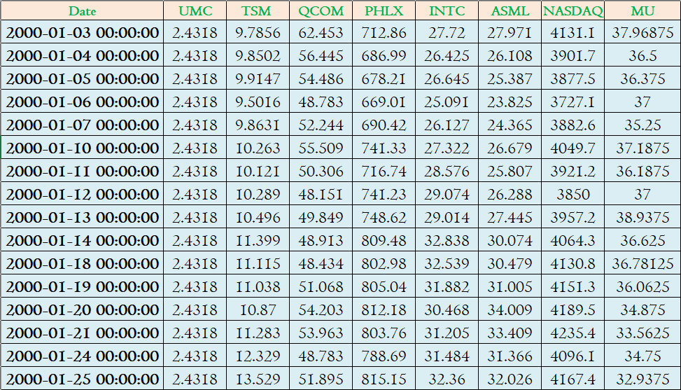
I have formatted and collated the downloaded data into one excel file “StockData.xlsx”

我已经将下载的数据格式化并整理到一个Excel文件“ StockData.xlsx”中

Last 20 years stock price data — from Jan 2000 until Aug 2020

最近20年的股价数据-从2000年1月到2020年8月

Step 3- We will import the packages pandas, matplotlib, seaborn and statsmodels packages which we are going to use for our analysis.

第3步-我们将导入将用于分析的软件包pandas，matplotlib，seaborn和statsmodels软件包。

import pandas as  pd
import matplotlib.pyplot as plt
import seaborn as sns
from statsmodels.stats.outliers_influence import variance_inflation_factor

Step 4- Read the full data sample data excel file into the PandasDataframe called “data”. Further, we will replace the index with the date column

步骤4-将完整的数据样本数据excel文件读入称为“ data”的PandasDataframe中。 此外，我们将索引替换为日期列

data=pd.read_excel("StockData.xlsx")
data.set_index("Date", inplace= True)

I will not focus on preliminary data quality checks like blank values, outliers, etc. and respective correction approach in this article, and assuming that there are no data series related to the discrepancy.

在本文中，我将不着重于初步的数据质量检查，例如空白值，离群值等，以及相应的校正方法，并假设没有与差异有关的数据系列。

Step 5- One of the best places to start understanding the relationship between the independent variable is the correlation between the variables. In the below code, heatmap of the correlation is plotted using .corr method in Pandas.

步骤5-开始了解自变量之间的关系的最佳位置之一是变量之间的相关性。 在下面的代码中，在Pandas中使用.corr方法绘制了相关的热图。

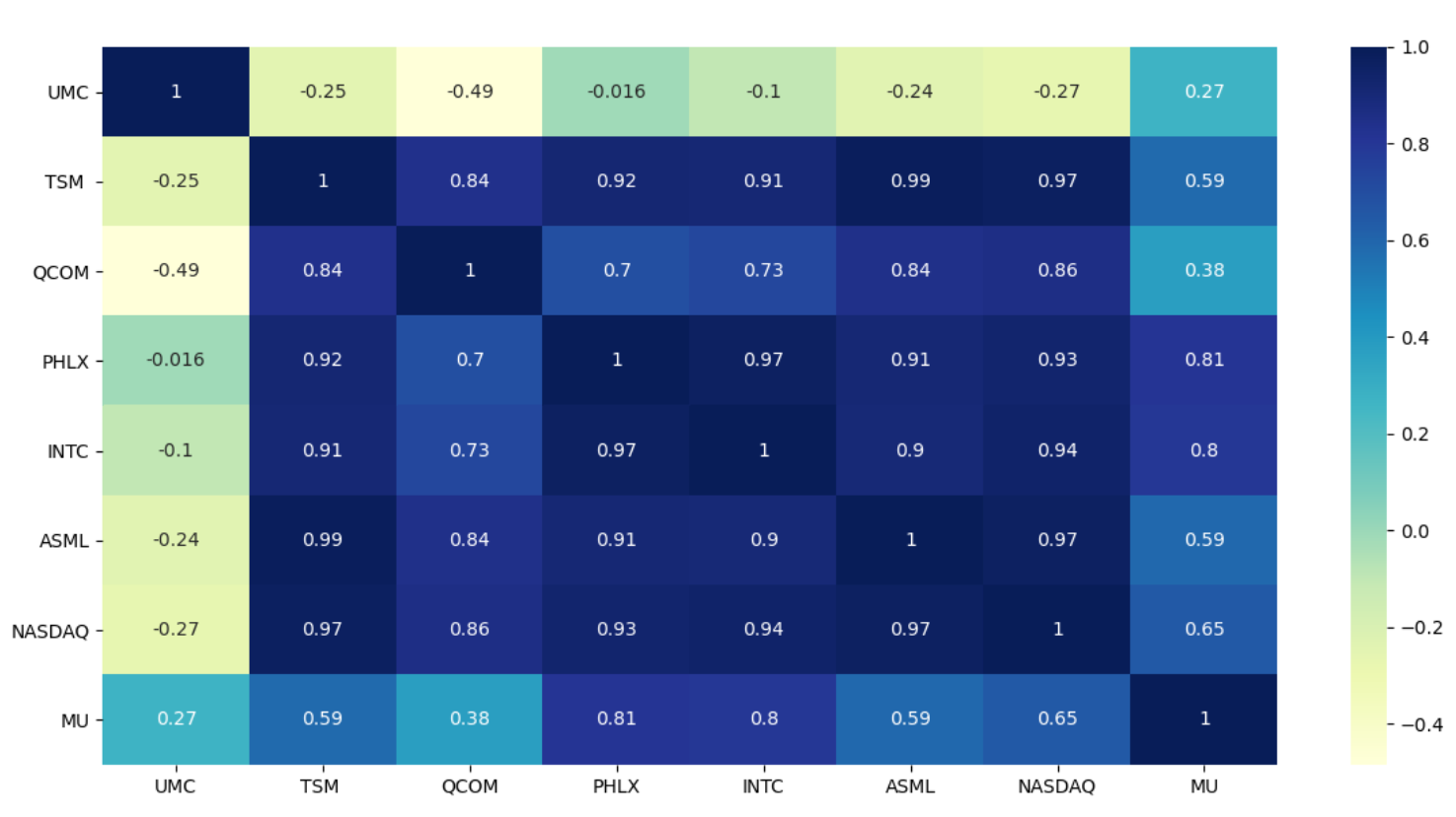
sns.heatmap(data.corr(), annot=True, cmap="YlGnBu")
plt.show()

Correlation heatmap, as shown below, provides us with a visual depiction of the relationship between the variables. Now, we do not want a set of independent variables which has a more or less similar relationship with the dependent variables. For example, TSM and Nasdaq index has a correlation coefficient of 0.99 and 0.97 with ASML respectively. Including both TSM and NASDAQ may not improve the prediction accuracy as they have a similar relationship with the dependent variable, ASML stock price.

如下所示，相关热图为我们提供了变量之间关系的直观描述。 现在，我们不希望有一组与因变量具有或多或少相似关系的自变量。 例如，TSM和Nasdaq指数与ASML的相关系数分别为0.99和0.97。 同时包含TSM和NASDAQ可能不会提高预测准确性，因为它们与因变量ASML股票价格具有相似的关系。

Step 6- Before we start dropping the redundant independent variables, let us check the Variance inflation factor (VIF) among the independent variables. VIF quantifies the severity of multicollinearity in an ordinary least squares regression analysis. It provides an index that measures how much the variance (the square of the estimate’s standard deviation) of an estimated regression coefficient is increased because of collinearity. I will encourage you all to read the Wikipedia page on Variance inflation factor to gain a good understanding of it.

第6步-在开始删除冗余自变量之前，让我们检查自变量之间的方差膨胀因子 ( VIF )。 VIF在普通最小二乘回归分析中量化多重共线性的严重性。 它提供了一个指标，用于衡量由于共线性而导致估计的回归系数的方差(估计的标准偏差的平方)增加了多少。 我鼓励大家阅读Wikipedia页面上关于方差膨胀因子的知识 ，以更好地理解它。

In the below code we calculate the VIF of each independent variables and print it. We will create a new DataFrame without ASML historical stock prices as we aim is to determine the VIF among the potential independent variables.

在下面的代码中，我们计算每个独立变量的VIF并将其打印出来。 我们将创建一个没有ASML历史股价的新DataFrame，因为我们的目的是确定潜在自变量中的VIF。

X=data.drop(["ASML"], axis=1)
vif = pd.DataFrame()
vif["features"] = X.columns
vif["vif_Factor"] = [variance_inflation_factor(X.values, i) for i in range(X.shape[1])]
print(vif)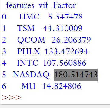

In general, we should aim for the VIF of less than 10 for the independent variables. We have seen from the heatmap earlier that TSM and NASDAQ have similar correlation coefficient with ASML and the same is also reflecting with high VIF indicator.

通常，我们应将自变量的VIF设置为小于10。 从较早的热图中我们可以看到，TSM和NASDAQ与ASML具有相似的相关系数，并且在高VIF指标下也反映出相同的相关系数。

Based on our understanding from heatmap and VIF result let us drop NASDAQ (as highest VIF) as a potential candidate for the independent variable for our model and re-evaluate the VIF.

根据我们对热图和VIF结果的理解，让我们放弃纳斯达克(作为最高VIF)作为模型自变量的潜在候选者，然后重新评估VIF。

X=data.drop(["ASML","NASDAQ"], axis=1)
vif = pd.DataFrame()
vif["features"] = X.columns
vif["vif_Factor"] = [variance_inflation_factor(X.values, i) for i in range(X.shape[1])]
print(vif)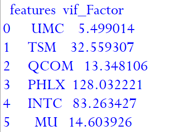

We can see that on removing the NASDAQ, VIF of few other potential independent also decreased.

我们可以看到，在删除纳斯达克后，其他潜在独立股的VIF也降低了。

Selecting the right combination of independent variables is a bit of experience along with trial and error VIF checking with different permutations. TSMC is a leading semiconductor foundry in the world and as a customer of ASML has a strong influence on ASML’s business. Considering this aspect, I will drop “INTC” and “PHLX” and re-evaluate the VIF for the remaining variables.

选择正确的自变量组合会带来一些经验，并会尝试使用具有不同排列的反复试验VIF。 台积电是全球领先的半导体代工厂，作为ASML的客户，对ASML的业务有深远的影响。 考虑到这方面，我将删除“ INTC”和“ PHLX”，并对剩余变量重新评估VIF。

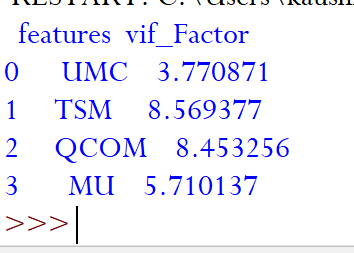
As we can see that after two iterations we have VIF of all the remaining variables less than 10. We have removed the variables with multicollinearity and have identified the list of independent variables which are relevant for predicting the stock prices of ASML.

正如我们看到的那样，经过两次迭代，我们剩下的所有变量的VIF都小于10。我们删除了具有多重共线性的变量，并确定了与预测ASML股价相关的自变量列表。

I hope, in selecting the right sets of the independent variable for your machine learning models, you will find the approach explained in this program helpful.

我希望，在为您的机器学习模型选择正确的独立变量集时，您会发现此程序中介绍的方法会有所帮助。

If you like this article then you may also like Machine Learning and Supply Chain Management: Hands-on Series

如果您喜欢本文，那么您可能也喜欢机器学习和供应链管理：动手系列

Disclaimer — This article is written for educational purpose only. Do not make any actual stock buying, selling or any financial transaction based on the independent variables identified in this article.

免责声明—本文仅用于教育目的。 不要根据本文确定的独立变量进行任何实际的股票买卖，金融交易。

翻译自: https://towardsdatascience.com/how-to-identify-the-right-independent-variables-for-machine-learning-supervised-algorithms-439986562d32

机器学习 多变量回归算法