深度学习强化学习策略迭代-CSDN博客

有关深层学习的FAU讲义 (FAU LECTURE NOTES ON DEEP LEARNING)

These are the lecture notes for FAU’s YouTube Lecture “Deep Learning”. This is a full transcript of the lecture video & matching slides. We hope, you enjoy this as much as the videos. Of course, this transcript was created with deep learning techniques largely automatically and only minor manual modifications were performed. Try it yourself! If you spot mistakes, please let us know!

这些是FAU YouTube讲座“ 深度学习 ”的讲义。 这是演讲视频和匹配幻灯片的完整记录。 我们希望您喜欢这些视频。 当然，此成绩单是使用深度学习技术自动创建的，并且仅进行了较小的手动修改。 自己尝试！ 如果发现错误，请告诉我们！

导航 (Navigation)

Previous Lecture / Watch this Video / Top Level / Next Lecture

上一个讲座 / 观看此视频 / 顶级 / 下一个讲座

Image for post — Also, Mario isn’t save from Reinforcement Learning. Image created using gifify. Source: YouTube.

Welcome back to deep learning! So today, we want to go deeper into reinforcement learning. The concept that we want to explain today is going to be policy iteration. It tells us how to make better policies towards designing strategies for winning games.

欢迎回到深度学习！因此，今天，我们想更深入地学习强化学习。我们今天要解释的概念将是策略迭代。它告诉我们如何制定更好的策略来设计获胜游戏的策略。

So, let’s have a look at the slides that I have here for you. So it’s the third part of our lecture and we want to talk about policy iteration. Now, before we had this action-value function that somehow could assess the value of an action. Of course, this now has also to depend on the state t. This is essentially our — you could say Oracle — that tries to predict the future reward g subscript t. It depends on following a certain policy that describes how to select the action and the resulting state. Now, we can also find an alternative formulation here. We introduce the state-value function. So, previously we had the action-value function that told us how valuable a certain action is. Now, we want to introduce the state-value function that tells us how valuable a certain state is. Here, you can see that it is formalized in a very similar way. Again, we have some expected value over our future reward. This is now, of course, dependent on the state. So, we kind of leave away the dependency on the action and we only focus on the state. You can now see that this is the expected value of the future reward with respect to the state. So, we want to marginalize the actions. We don’t care about what the influence of the action is. We just want to figure out what the value of a certain state is.

因此，让我们来看一下我为您准备的幻灯片。因此，这是我们讲座的第三部分，我们想谈谈策略迭代。现在，在我们有了这个动作值函数之前，它可以某种方式评估一个动作的值。当然，现在这也必须取决于状态t。本质上，这就是我们(您可以说是Oracle)试图预测未来奖励g下标t。这取决于是否遵循描述了如何选择操作和结果状态的特定策略。现在，我们也可以在这里找到替代公式。我们介绍状态值函数。因此，以前我们有动作值函数来告诉我们某个动作的价值。现在，我们要介绍状态值函数，该函数告诉我们某个状态的价值。在这里，您可以看到它以非常相似的方式形式化。同样，我们对未来的奖励有一些期望值。现在，这当然取决于状态。因此，我们有点放弃了对动作的依赖，而只关注状态。您现在可以看到，这是关于状态的未来奖励的期望值。因此，我们想将行动边缘化。我们不在乎动作的影响是什么。我们只想弄清楚某个状态的值是什么。

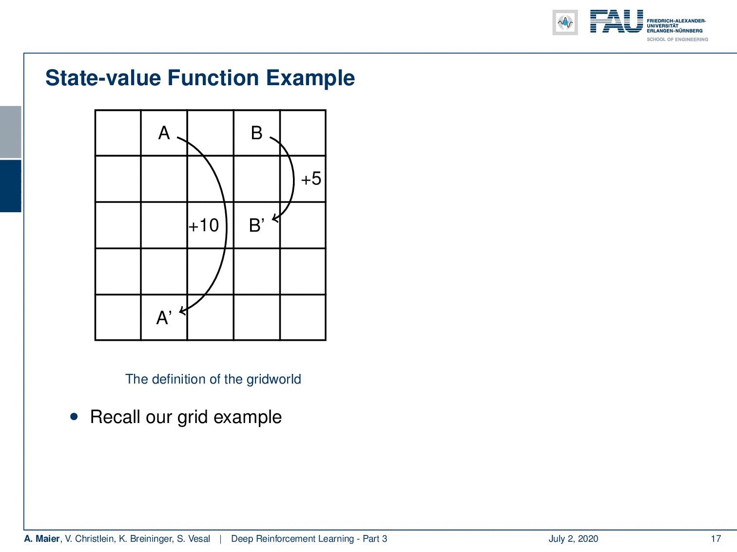
We can actually compute this. So, we can also do this for our grid example. If you recall this one, you remember that we had the simple game where you had A and B that were essentially the locations on the grid that would then teleport you to A’ and B’. Once, you arrive at A’ and B’, you get a reward. For A’ its +10 and for B’ it’s +5. Whenever you try to leave the board, you get a negative reward. Now, we can play this game and compute the state-value function. Of course, we can do this under the uniform random policy because we don’t have to know anything about the game. If we play the random uniform policy, we can simply choose actions, play this game for a certain time, and then we are able to compute these state values according to the previous definition. You can see that the edge tiles, in particular, in the bottom, they even have a negative value. Of course, they can have negative values because if you are in the edge tiles, we find -1.9 and -2.0 and the bottom. At the corner tiles, there is a 50% likelihood that you will try to leave the grid. In these two directions, you will, of course, generate a negative reward. So, you can see that we have states that are much more valuable. You can see if you look at the positions where A and B are located, they have a very high value. So A has an expected future reward of 8.8 and the tile with B has an expected future reward of 5.3. So, these are really good states. So, you could say with this state value, we have somehow learned something about our game. So, you could say “Okay, maybe we can use this.” We can now use the greedy action selection on this state value. So let’s define a policy and this policy is now selecting always the action that leads into a state of a higher value. If you do so, you have a new policy. If you play with this new policy you see you have a better policy.

我们实际上可以计算出这一点。因此，我们也可以针对我们的网格示例执行此操作。如果您还记得这一本书，您会记得我们有一个简单的游戏，您拥有A和B，它们实际上是网格上的位置，然后将您传送到A'和B'。一旦到达A'和B'，您将获得奖励。 A'为+ 10，B'为+5。每当您尝试离开董事会时，您都会获得负面奖励。现在，我们可以玩这个游戏并计算状态值函数。当然，我们可以在统一的随机策略下执行此操作，因为我们不必了解任何游戏。如果我们执行随机统一策略，则可以简单地选择动作，玩一定时间的游戏，然后能够根据先前的定义计算这些状态值。您可以看到，尤其是在底部的边缘瓦片，甚至具有负值。当然，它们可以具有负值，因为如果您在边缘切片中，我们会发现-1.9和-2.0以及底部。在墙角砖处，您有50％的可能性尝试离开网格。在这两个方向上，您当然会产生负面奖励。因此，您可以看到我们的状态更有价值。您可以查看一下A和B所在的位置，它们的值很高。因此，A的预期未来回报为8.8，而B的区块的预期未来回报为5.3。因此，这些都是非常好的状态。因此，您可以说使用此状态值，我们已经从某种程度上了解了我们的游戏。因此，您可以说“好吧，也许我们可以使用它。” 现在，我们可以在此状态值上使用贪婪动作选择。因此，让我们定义一个策略，该策略现在总是选择导致更高价值状态的操作。如果这样做，您将有一个新政策。如果您使用这项新政策，将会发现您有更好的政策。

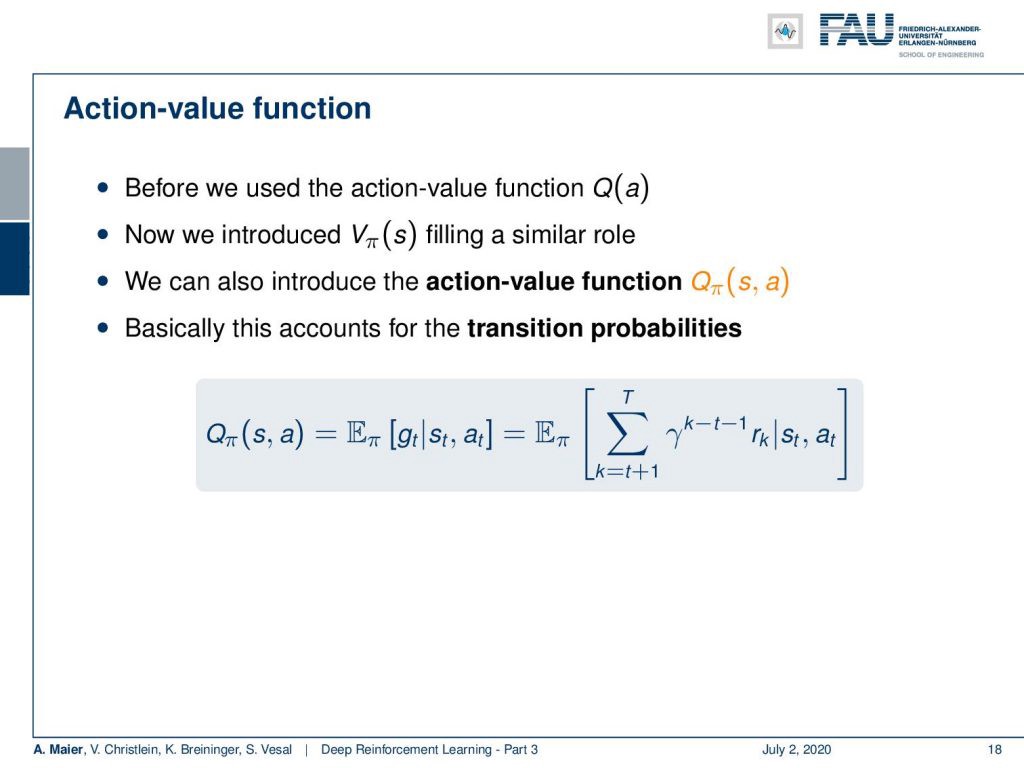
So, we can now relate this to the action-value function that we used before. We somehow introduced the state-value function in a similar role. So, we can now see that we can introduce an action-value function that is Q subscript policy of s and a, i.e., of the state and the action. This then basically accounts for the transition probabilities. So, you can now compute your Q policy of state and action as the expected value of the future rewards given the state and the action. You can compute this in a similar way. Now, you get an expected future reward for every state and for every action.

因此，我们现在可以将其与之前使用的动作值函数相关联。我们以某种方式引入了状态值函数。因此，现在我们可以看到可以引入一个动作值函数，该函数是s和a的Q下标策略，即状态和动作的Q下标策略。然后，这基本上说明了转移概率。因此，您现在可以将状态和操作的Q策略计算为给定状态和操作的未来奖励的期望值。您可以用类似的方式进行计算。现在，您将为每个州和每个行动获得预期的未来回报。

Are all of these value functions created equal? No. There can only be one optimal state value function. We can show its existence without referring to a specific policy. So, the optimal state-value function is simply the maximum of all state-value functions with the best policy. So, the best policy will always produce the optimal state-value function. Now, we can also define the optimal action-value function. This can now be related to our optimal state-value function. We can see that the optimal action-value function is given as the expected reward in the next step plus our discount factor times the optimal state-value function. So, if we know the optimal state-value function, then we can also derive the optimal action-value function. So, they are related to each other.

创建的所有这些价值函数是否相等？不可以。只能有一个最佳状态值函数。我们可以在不参考特定政策的情况下证明其存在。因此，最佳状态值函数只是具有最佳策略的所有状态值函数中的最大值。因此，最佳策略将始终产生最佳状态值函数。现在，我们还可以定义最佳作用值函数。现在，这可以与我们的最佳状态值函数相关。我们可以看到，最佳行动价值函数作为下一步的预期报酬加上我们的折扣系数乘以最佳状态价值函数得出。因此，如果我们知道最佳状态值函数，那么我们也可以导出最佳动作值函数。因此，它们彼此相关。

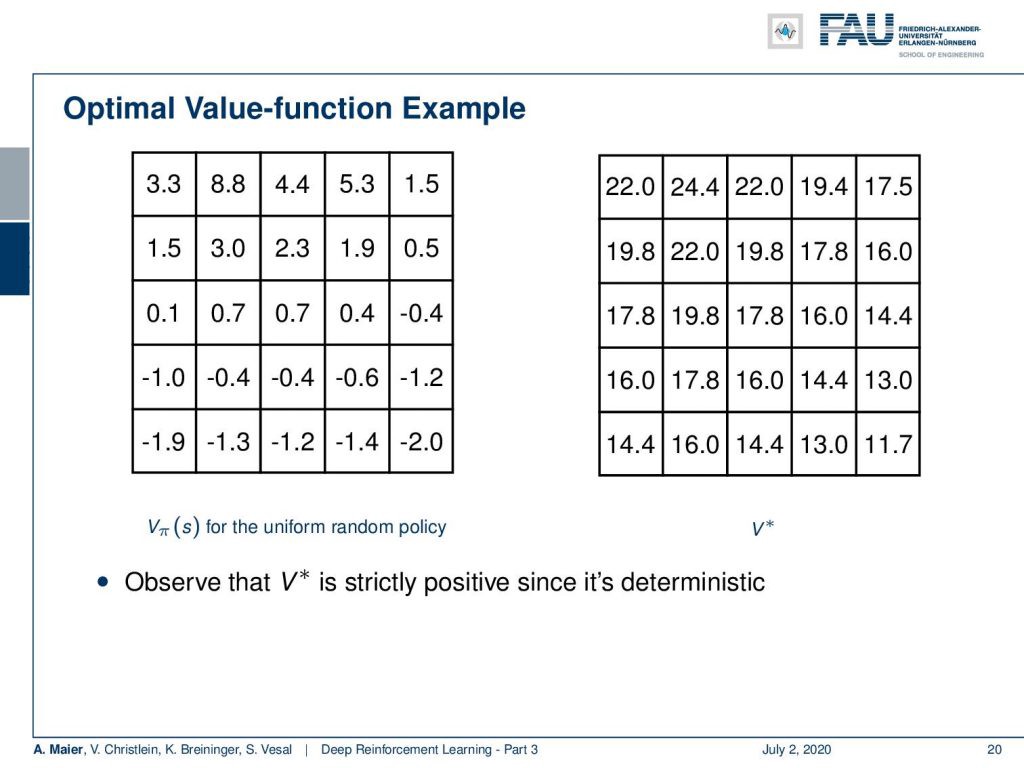
So, this was the state-value function for the uniform random policy. I can show you the optimal V*, i.e., the optimal state-value function. You see that this has much higher values, of course, because we have been optimizing for this. You also observe that the optimal state-value function is strictly positive because we are in a deterministic setting here. So, very important observation: In a deterministic setting, the optimal state-value function will be strictly positive.

因此，这是统一随机策略的状态值函数。我可以向您展示最佳V *，即最佳状态值函数。您会看到它的值当然更高，因为我们一直在为此进行优化。您还会观察到最佳状态值函数严格为正，因为我们在这里处于确定性设置。因此，非常重要的观察：在确定性设置中，最佳状态值函数将严格为正。

Now, we can also order policies. We have to determine what is a better policy. We can order them with the following concept: A better policy π is better than a policy π’ if and only if the state values of π are all higher than the state values that you obtain with π’ for all states in the set of states. If you do this, then any policy that returns the optimal state-value function is an optimal policy. So, you see that it’s only one optimal state-value function, but there might be more than one optimal policy. So, there could be two or three different policies that result in the same optimal state-value function. So, if you know either the optimal state-value or the optimal action-value function, then you can directly obtain an optimal policy by greedy action selection. So, if you know the optimal state values and if you have complete knowledge about all the actions and so on, then you can always get the optimal policy by a greedy action selection.

现在，我们还可以订购保单。我们必须确定什么是更好的政策。我们可以使用以下概念对它们进行排序：当且仅当π的状态值都高于对状态集中的所有状态使用π'获得的状态值时，更好的策略π才比策略π'更好。。如果执行此操作，则返回最佳状态值函数的任何策略都是最佳策略。因此，您看到它只是一个最佳状态值函数，但是可能有不止一个最佳策略。因此，可能有两个或三个不同的策略导致相同的最佳状态值函数。因此，如果您知道最佳状态值或最佳动作值函数，则可以通过贪婪的动作选择直接获得最佳策略。因此，如果您知道最佳状态值，并且对所有动作等都有完整的了解，那么您总是可以通过贪婪的动作选择来获得最佳策略。

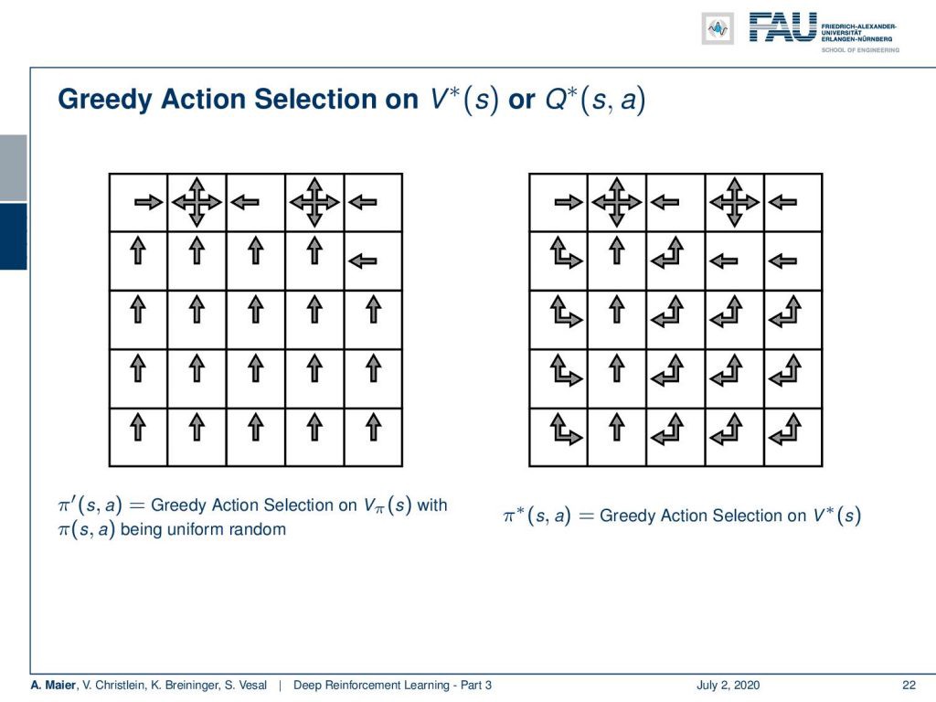
So, let’s have a look at how this would then actually result in terms of policies. Now, greedy action selection on the optimum state-value function or the optimal action-value function would lead to the optimal policy. Well, you see here on the left inside is greedy action selection on the uniform random state-value function. So, what we’ve computed earlier in this video. You can, of course, choose your action in a way that you have the next state being a state of higher value and you end up with this kind of policy. Now, if you do the same thing on the optimal state value function, you can see that we essentially emerge with a very similar policy. You see a couple of differences. In fact, you don’t always have to move up like shown on the left-hand side. So, you can also move left or up on several occasions. You can actually choose the action at each of these squares that are indicated with multiple arrows with equal probability. So, if there’s an up and left arrow, you can choose either action and you would still have an optimal policy. So, this would be the optimal policy that is created by a greedy action selection on the optimal state value function.

因此，让我们看一下这在政策方面的实际结果。现在，在最佳状态值函数或最佳动作值函数上进行贪婪的行为选择将导致最优策略。好吧，您在这里看到的左侧是统一随机状态值函数上的贪婪动作选择。因此，我们在本视频的前面已经进行了计算。当然，您可以选择一种行动，使下一个状态成为具有较高价值的状态，并最终得到这种策略。现在，如果您在最佳状态值函数上执行相同的操作，则可以看到我们在本质上出现了非常相似的策略。您会看到一些差异。实际上，您不必总是像左侧所示那样向上移动。因此，您也可以在几种情况下向左或向上移动。实际上，您可以在这些正方形的每个正方形上选择动作，这些正方形均以相等的概率由多个箭头指示。因此，如果有一个向上和向左的箭头，则您可以选择任一操作，并且仍将具有最佳策略。因此，这将是通过对最佳状态值函数进行贪婪操作选择而创建的最佳策略。

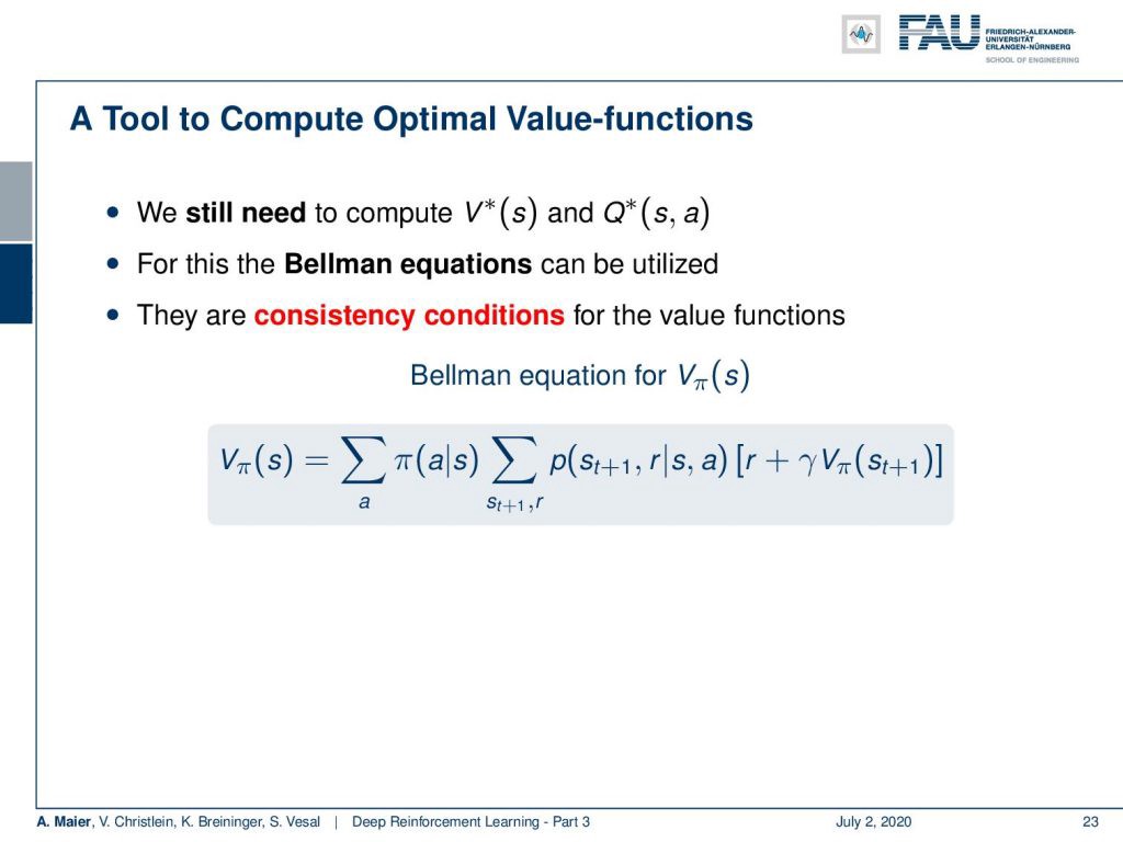
Now, the big question is: “How can we compute optimal value functions?” We still have to determine this optimal state-value function and the optimal action-value function. In order to do this, there are the Bellman equations. They are essentially consistency conditions for value functions. So, this is the example of the state-value function. You can see that you have to sum over all the different actions that are determined by your policy. So, we want to marginalize out the influence of the actual action. Of course, depending on what action you would choose, you would generate different states and different rewards. So, you also sum over the different states and the respective rewards here and multiply the probability of the states with the actual reward plus the discounted state-value function of the next state. So in this way, you can determine the state-value function. You see that there is this dependency between the current state and the next state in this computation.

现在，最大的问题是：“我们如何计算最优值函数？” 我们仍然必须确定此最佳状态值函数和最佳动作值函数。为此，需要使用Bellman方程。它们本质上是价值函数的一致性条件。因此，这是状态值函数的示例。您可以看到您必须对由策略确定的所有不同操作进行汇总。因此，我们想边缘化实际行动的影响。当然，根据您选择的操作，您将产生不同的状态和不同的奖励。因此，您还可以在此处汇总不同状态和相应的奖励，然后将状态的概率与实际奖励以及下一个状态的折扣状态值函数相乘。因此，可以通过这种方式确定状态值函数。您会看到在此计算中，当前状态和下一个状态之间存在这种依赖性。

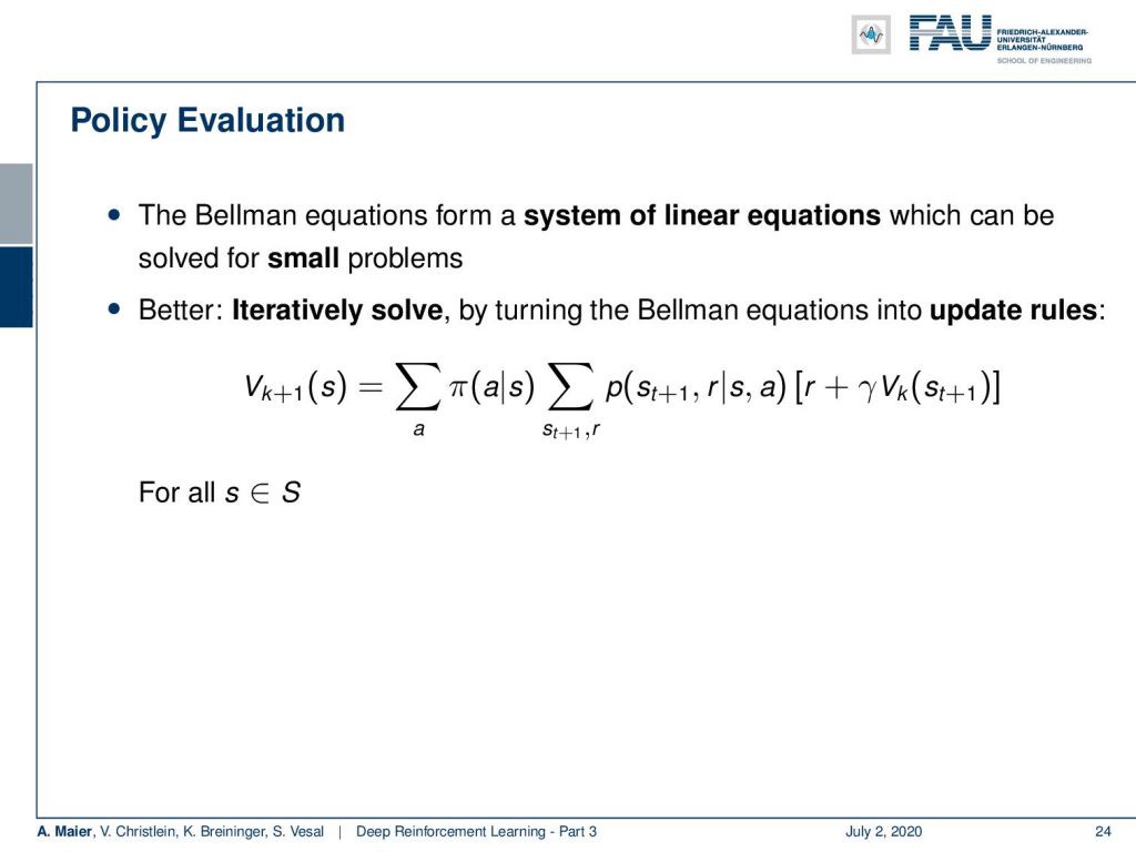
This means you can either write this up as a system of linear equations and actually solve this for small problems. But what is even better is that you iteratively solve this by turning the Bellman equations into update rules. So, you see now that we can generate a new value function k+1 for the current state if we simply apply the Bellman equation. So, we have to compute all of the different actions. We have to evaluate actually all of the different actions given the state. Then, we determine all the next future states and the next future rewards and update this according to our previous state-value function. Of course, we do this for all the states s. Then, we have an updated state-value function. Okay. So, this is an interesting observation. If we have some policy, we can actually run those updates.

这意味着您既可以将其写为线性方程组，也可以解决小问题。但是更好的是，您可以通过将Bellman方程式转换为更新规则来迭代地解决此问题。因此，您现在看到，只要简单地应用Bellman方程，就可以为当前状态生成一个新的值函数k + 1。因此，我们必须计算所有不同的动作。实际上，我们必须评估给定状态下的所有不同操作。然后，我们确定所有下一个未来状态和下一个未来奖励，并根据我们先前的状态值函数进行更新。当然，我们对所有州都这样做。然后，我们有一个更新的状态值函数。好的。因此，这是一个有趣的观察。如果有一些政策，我们实际上可以运行这些更新。

This leads us then to the concept of policy improvement. This policy iteration is what we actually want to talk about in this video. So, we can use now our state-value function to guide our search for good policies. Then, we update the policy. So, if we use the greedy action selection for an update of the state-value function, then this also means that we simultaneously update our policy because the greedy action selection on our state value will always result in different actions if we change the state values. So, any change or update in the state values will also imply an updated policy in case of greedy action selection because we directly linked them together. So this then means that we can iterate the evaluation of a greedy policy on our state-value function. We stop iterating if our policy stops changing. So, this way we can update the state values and with the update of the state values, we immediately also update our policy. Is this actually guaranteed to work?

这使我们想到了政策改进的概念。此政策迭代是我们在本视频中实际要讨论的内容。因此，我们现在可以使用状态值函数来指导我们寻找良好的政策。然后，我们更新该政策。因此，如果我们使用贪婪动作选择来更新状态值函数，那么这也意味着我们同时更新了我们的策略，因为如果更改状态值，对我们状态值的贪婪动作选择将始终导致不同的动作。因此，在选择贪婪操作的情况下，状态值的任何更改或更新也都意味着更新了策略，因为我们直接将它们链接在一起。因此，这意味着我们可以根据状态值函数迭代对贪婪策略的评估。如果我们的政策停止更改，我们将停止迭代。因此，通过这种方式，我们可以更新状态值，并且随着状态值的更新，我们也立即更新了策略。这真的可以保证工作吗？

Well, there’s the policy improvement theorem. If we consider changing a single action a subscript t and state s subscript t, following a policy. Then, in general, if we have a higher action-value function, the state value for all states s increases. This means that we have a better policy. So, the new policy is then a better policy. This would then also imply that we also get a better state value because we generate a higher future reward in all of the states. This means that also the state-value function must have been increased. If we only greedy select, then we will always produce a higher action value than the state value before the convergence. So, we iteratively updating the state value using greedy action selection is really a guaranteed concept here in order to improve our state values. We terminate if the policy no longer changes. One last remark: if we don’t loop over all the states in our state space for the policy evaluation but update the policy directly, this is then called value iteration. Okay. So, you have seen now in this video how we can use the state value function in order to describe the expected future reward of a specific state. We have seen that if we do greedy action selection on the state-value function, we can use this to generate better policies. If we follow a better policy, then also our state-value function will increase. So if we follow this concept, we end up in the concept of policy iteration. So with every update of the state value function where you find higher state values, you also find a better policy. This means that we can improve our policy step-by-step by the concept of policy iteration. Okay. So, this was a very first learning algorithm in the concept of reinforcement learning.

好吧，这里有一个政策改进定理。如果我们考虑按照策略更改单个动作，则下标t和状态s下标t。然后，通常，如果我们具有较高的动作值函数，则所有状态s的状态值都会增加。这意味着我们有更好的政策。因此，新政策才是更好的政策。这也意味着我们还可以获得更好的州价值，因为我们在所有州中产生了更高的未来回报。这意味着还必须增加状态值函数。如果我们只是贪婪地选择，那么我们总是会产生比收敛之前的状态值更高的动作值。因此，为了提高状态值，在此使用贪婪动作选择迭代更新状态值确实是一个有保证的概念。如果政策不再更改，我们将终止。最后一句话：如果我们不循环状态空间中的所有状态以进行策略评估，而是直接更新策略，则这称为值迭代。好的。因此，您现在已经在该视频中看到了如何使用状态值函数来描述特定状态的预期未来回报。我们已经看到，如果我们对状态值函数进行贪婪的动作选择，则可以使用它来生成更好的策略。如果我们遵循更好的政策，那么我们的状态值函数也会增加。因此，如果遵循这个概念，我们最终会遇到策略迭代的概念。因此，在每次更新状态值功能时，您都会找到更高的状态值，从而找到更好的策略。这意味着我们可以通过策略迭代的概念逐步改进策略。好的。因此，这是强化学习概念中的第一个学习算法。

But of course, this is not everything. There are a couple of drawbacks and we’ll talk about more concepts on how to improve actually our policies in the next video. There are a couple more. So, we will present them and also talk a bit about the drawbacks of the different versions. So, I hope you liked this video and we will talk a bit more in the next couple of videos about reinforcement learning. So, stay tuned and hope to see you in the next video. Bye-bye!

但是，当然，这还不是全部。有两个缺点，我们将在下一个视频中讨论更多有关如何实际改善政策的概念。还有更多。因此，我们将介绍它们，并讨论不同版本的缺点。因此，我希望您喜欢这个视频，在接下来的两节关于强化学习的视频中，我们将进一步讨论。因此，请继续关注并希望在下一个视频中见到您。再见！

If you liked this post, you can find more essays here, more educational material on Machine Learning here, or have a look at our Deep Learning Lecture. I would also appreciate a follow on YouTube, Twitter, Facebook, or LinkedIn in case you want to be informed about more essays, videos, and research in the future. This article is released under the Creative Commons 4.0 Attribution License and can be reprinted and modified if referenced. If you are interested in generating transcripts from video lectures try AutoBlog.

如果你喜欢这篇文章，你可以找到这里更多的文章，更多的教育材料，机器学习在这里，或看看我们的深入学习讲座。如果您希望将来了解更多文章，视频和研究信息，也欢迎关注YouTube ， Twitter ， Facebook或LinkedIn 。本文是根据知识共享4.0署名许可发布的，如果引用，可以重新打印和修改。如果您对从视频讲座中生成成绩单感兴趣，请尝试使用AutoBlog 。