吴恩达《机器学习》编程作业——machine-learning-ex1：线性回归

最新推荐文章于 2019-04-24 16:01:30 发布

weixin_30555753

最新推荐文章于 2019-04-24 16:01:30 发布

阅读量472

点赞数

文章标签：数据结构与算法人工智能操作系统

原文链接：http://www.cnblogs.com/lky-learning/p/10459374.html

版权

❄❄❄❄❄❄❄❄【回到目录】❄❄❄❄❄❄❄❄

本次编程作业中，需要完成的代码有如下几部分：

[⋆] warmUpExercise.m - Simple example function in Octave/MATLAB
[⋆] plotData.m - Function to display the dataset
[⋆] computeCost.m - Function to compute the cost of linear regression
[⋆] gradientDescent.m - Function to run gradient descent
[†] computeCostMulti.m - Cost function for multiple variables
[†] gradientDescentMulti.m - Gradient descent for multiple variables
[†] featureNormalize.m - Function to normalize features
[†] normalEqn.m - Function to compute the normal equations

1 warmUpExercise.m --- Octave/MATLAB的简单函数

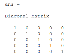
在文件warmUpExercise.m中，您将看到Octave / MATLAB函数的概要。通过填写以下代码修改它以返回5 x 5单位矩阵：

function A = warmUpExercise()
%WARMUPEXERCISE Example function in octave
%   A = WARMUPEXERCISE() is an example function that returns the 5x5 identity matrix
% ============= YOUR CODE HERE ==============

A = eye(5);

% ========================================== end

完成之后，运行ex1.m，就可以看到类似于以下内容的输出：

2 plotData.m --- 将数据绘制成图像

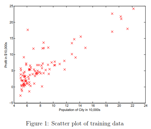
绘制图形可以帮助我们可视化数据。对于此数据集，我们可以使用散点图来绘制数据，因为它只有收益和人口两个数据（在现实生活中很多问题都是多维数据表示，并不能绘制成二维图）。

加载数据：

data = load('ex1data1.txt');
X = data(:, 1); y = data(:, 2);
m = length(y); % number of training examples

接下来，该程序调用plotData子函数来绘制数据的散点图。你的工作是完成plotData.m函数来绘制图像;，修改代码：

function plotData(x, y)

% ====================== YOUR CODE HERE ======================
% Hint: 您可以在绘图中使用'rx'选项，使标记显示为红色十字。
%       此外，您可以使用plot（...，'rx'，'MarkerSize'，10）
%       使标记更大

figure; % 打开一个新的数字窗口
plot(x, y, 'rx','MarkerSize', 10);    %r代表red； x 代表十字标记 ；10是标记的大小
ylabel('Profit in $10,000s');          %加y轴的标签
xlabel('Population of City in 10,000s');
% ============================================================
end

【plot( )函数的使用可以参考该文档】

运行ex1.m之后，你可以看到Figure 1。

3 computeCost.m --- 计算代价函数

线性回归的目的就是最小化代价函数：

其中假设函数h_θ(x)是一个线性模型：h_θ(x) = θ^T x = θ₀ + θ₁x₁。

当您执行梯度下降从而最小化成本函数J（θ）时，通过计算成本cost有助于监视是否收敛。在本节中，您将实现一个计算J（θ）的函数，以便检查梯度下降实现的收敛性。

function J = computeCost(X, y, theta)
%COMPUTECOST Compute cost for linear regression
%   J = COMPUTECOST(X, y, theta) computes the cost of using theta as the
%   parameter for linear regression to fit the data points in X and y

% Initialize some useful values
m = length(y); % number of training examples

% You need to return the following variables correctly 

% ====================== YOUR CODE HERE ======================
% Instructions: Compute the cost of a particular choice of theta
%               You should set J to the cost.

J = (1/(2*m))*sum(((X*theta) - y).^2)

% =========================================================================

end

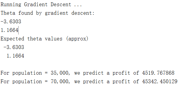
完成该子程序后，ex1.m中将使用零初始化的 θ 运行computeCost，您将该结果：　

4 gradientDescent.m --- 运行梯度下降

接下来你的任务是完成gradientDescent.m，从而实现梯度下降。在编程时，请确保你了解要优化的内容和正在更新的内容。请记住，代价函数J（θ）参数 θ 的函数，而不是X和y。也就是说，我们通过改变参数θ的值而不是通过改变X或y来最小化J（θ）。验证梯度下降是否正常工作的一种好方法是查看J（θ）的值，并检查它是否随着每一次迭代减小。如果正确实现了梯度下降和computeCost，则J（θ）的值不应该增加，并且应该在算法结束时收敛到稳定值。

我们通过调整参数 θ 的值从而最小化代价函数 J(θ)。通过batch梯度下降可以达到目的。在梯度下降中，每次迭代都执行下面的这个更新：

function [theta, J_history] = gradientDescent(X, y, theta, alpha, num_iters)
%GRADIENTDESCENT Performs gradient descent to learn theta
%   theta = GRADIENTDESCENT(X, y, theta, alpha, num_iters) updates theta by 
%   taking num_iters gradient steps with learning rate alpha

% Initialize some useful values
m = length(y); % number of training examples
J_history = zeros(num_iters, 1);

for iter = 1:num_iters

    % ====================== YOUR CODE HERE ======================
    % Instructions: Perform a single gradient step on the parameter vector
    %               theta. 
    %
    % Hint: While debugging, it can be useful to print out the values
    %       of the cost function (computeCost) and gradient here.
    %
    theta = theta-alpha*(1/m)*X'*(X*theta)-y);
    % ============================================================

    % Save the cost J in every iteration    
    J_history(iter) = computeCost(X, y, theta);

end

end

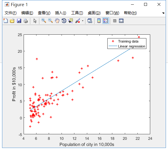
当你完成之后，完成后，ex1.m将使用最终参数来绘制线性逼近。结果应如下图所示：

5 featureNormalize.m --- 特征缩放

数据中，房屋大小的数量级约为卧室数量的1000倍。当特征相差几个数量级时，首先执行特征缩放可以使梯度下降更快地收敛。特征缩放的方式有以下几种：【特征缩放】（4.3节）

你的任务是完成featureNormalize.m

function [X_norm, mu, sigma] = featureNormalize(X)
%FEATURENORMALIZE Normalizes the features in X 
%   FEATURENORMALIZE(X) returns a normalized version of X where
%   the mean value of each feature is 0 and the standard deviation
%   is 1. This is often a good preprocessing step to do when
%   working with learning algorithms.

% You need to set these values correctly
X_norm = X;
mu = zeros(1, size(X, 2));
sigma = zeros(1, size(X, 2));

% ====================== YOUR CODE HERE ======================
% Instructions: First, for each feature dimension, compute the mean
%               of the feature and subtract it from the dataset,
%               storing the mean value in mu. Next, compute the 
%               standard deviation of each feature and divide
%               each feature by it's standard deviation, storing
%               the standard deviation in sigma. 
%
%               Note that X is a matrix where each column is a 
%               feature and each row is an example. You need 
%               to perform the normalization separately for 
%               each feature. 
%
% Hint: You might find the 'mean' and 'std' functions useful.
%       
mu = mean(X_norm);
sigma = std(X_norm );
X_norm(:,1) = ((X_norm(:,1)-mu(1)))./sigma(1);
X_norm(:,2) = ((X_norm(:,2)-mu(2)))./sigma(2);

% ============================================================

end

6 computeCostMulti.m --- 计算多变量的代价函数

之前已经完成了单变量线性回归中的计算代价函数和梯度下降，多变量的和单变量基本一致，唯一不同的是数据X矩阵中多了一个特征。

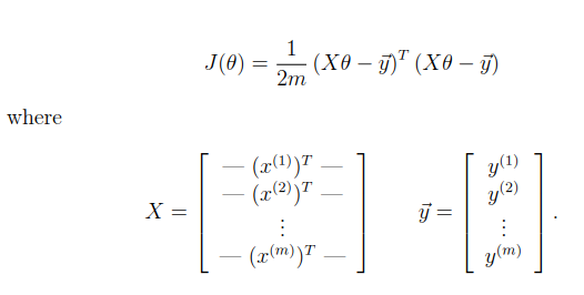
注意：在多变量的情况下，代价函数也可以使用以下的向量化形式编写：（向量化形式会使得计算更加高效）

function J = computeCostMulti(X, y, theta)
%COMPUTECOSTMULTI Compute cost for linear regression with multiple variables
%   J = COMPUTECOSTMULTI(X, y, theta) computes the cost of using theta as the
%   parameter for linear regression to fit the data points in X and y

% Initialize some useful values
m = length(y); % number of training examples

% You need to return the following variables correctly 
J = 0;

% ====================== YOUR CODE HERE ======================
% Instructions: Compute the cost of a particular choice of theta
%               You should set J to the cost.

J = (X*theta-y)'*(X*theta-y);   %或者 J = (1/(2*m))*sum(((X*theta) - y).^2);

% =========================================================================

end

7 gradientDescentMulti.m --- 多变量的梯度下降

function [theta, J_history] = gradientDescentMulti(X, y, theta, alpha, num_iters)
%GRADIENTDESCENTMULTI Performs gradient descent to learn theta
%   theta = GRADIENTDESCENTMULTI(x, y, theta, alpha, num_iters) updates theta by
%   taking num_iters gradient steps with learning rate alpha

% Initialize some useful values
m = length(y); % number of training examples
J_history = zeros(num_iters, 1);

for iter = 1:num_iters

    % ====================== YOUR CODE HERE ======================
    % Instructions: Perform a single gradient step on the parameter vector
    %               theta. 
    %
    % Hint: While debugging, it can be useful to print out the values
    %       of the cost function (computeCostMulti) and gradient here.
    %

    theta = theta - (alpha/m)*(X')*(X*theta - y);

    % ============================================================

    % Save the cost J in every iteration    
    J_history(iter) = computeCostMulti(X, y, theta);

end

end

8 normalEqn.m --- 正规方程

区别于迭代的方式，还可以用正规方程来求解：

使用此公式不需要任何特征缩放，可以在一次计算中得到一个精确的解决方案。

function [theta] = normalEqn(X, y)
%NORMALEQN Computes the closed-form solution to linear regression 
%   NORMALEQN(X,y) computes the closed-form solution to linear 
%   regression using the normal equations.

theta = zeros(size(X, 2), 1);

% ====================== YOUR CODE HERE ======================
% Instructions: Complete the code to compute the closed form solution
%               to linear regression and put the result in theta.
%
% ---------------------- Sample Solution ----------------------

theta = pinv(X'*X)*(X'*y)

% -------------------------------------------------------------

% ============================================================

end

如果这篇文章帮助到了你，或者你有任何问题，欢迎扫码关注微信公众号：一刻AI 在后台留言即可，让我们一起学习一起进步！

转载于:https://www.cnblogs.com/lky-learning/p/10459374.html

weixin_30555753

关注

0
点赞
踩
3

收藏

觉得还不错? 一键收藏
0
评论
吴恩达《机器学习》编程作业——machine-learning-ex1：线性回归

❄❄❄❄❄❄❄❄【回到目录】❄❄❄❄❄❄❄❄本次编程作业中，需要完成的代码有如下几部分：[⋆] warmUpExercise.m - Simple example function in Octave/MATLAB[⋆] plotData.m - Function to display the dataset[⋆] computeCost.m - Function to comp...
复制链接

扫一扫