Mathematica数据处理(10)--美化(下)

今天讲一下美化的最后一篇

其实还有两个函数没讲，分别是标签，和图例，我会另外讲的

那就直接开始讲吧

FrameLabel

GridLines

Plot[
 Sin[x], {x, 0, 10},
 Axes -> False,
 Frame -> {{True, False}, {True, False}},
 FrameLabel -> {{y, None}, {x, None}},
 RotateLabel -> False
 ]

注意:

(*RotateLabel使得标签不旋转*)
(*FrameLabel的也是{{left,right},{bottom,top}}*)

标签可以有四个位置可以放置

Manipulate[x, {x, 0, 1},
 FrameLabel -> {{"left label", "right label"}, {"bottom label","top label"}}]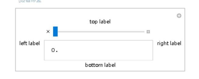

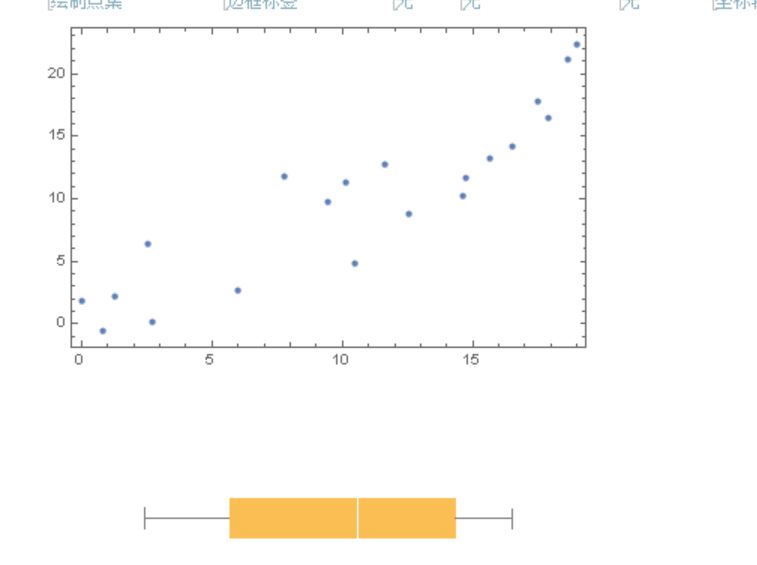
标签也不一定是文字，可以是任意的东西

data = Table[{i + RandomReal[{-3, 3}], i + RandomReal[{-4, 4}]}, {i, 
    1, 20}];
xlbl = BoxWhiskerChart[
   data[[All, 1]],
   BarOrigin -> Left,
   (*使得横着放*)
   Frame -> False,
   ImageSize -> 300
   ];
ListPlot[data, FrameLabel -> {{None, None}, {xlbl, None}}, 
 Axes -> False, Frame -> True]

得到下面的图

下面讲一下GridLines

Plot[Sin[x], {x, 0, 4 Pi},
 ImageSize -> 500,
 GridLines -> {{1, 2, 3}, Automatic}
 (*使用None就是不画*)
 ]

得到下面的图形

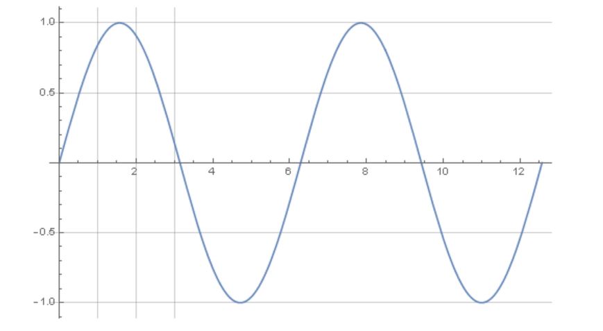
其中GridLines{{1,2,3},}表示在x=1，2，3的地方画线

系统默认的是网格线先画，有的时候会被隐藏，Method -> {"GridLinesInFront" -> True}可以使用这句话

(*在 某些情况下，网格线可能被隐藏*)
(*这时就要使用 Method\[Rule]{"GridLinesInFront"\[Rule]True}*)
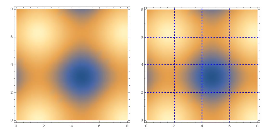
GraphicsRow[{
  DensityPlot[Sin[x] + Cos[y], {x, 0, 8}, {y, 0, 8}, 
   GridLines -> Automatic],
  
  DensityPlot[Sin[x] + Cos[y], {x, 0, 8}, {y, 0, 8}, 
   GridLines -> Automatic, 
   GridLinesStyle -> Directive[Blue, Dashed, Thick], 
   Method -> {"GridLinesInFront" -> True}]
  }, ImageSize -> 700]

得到下面的图

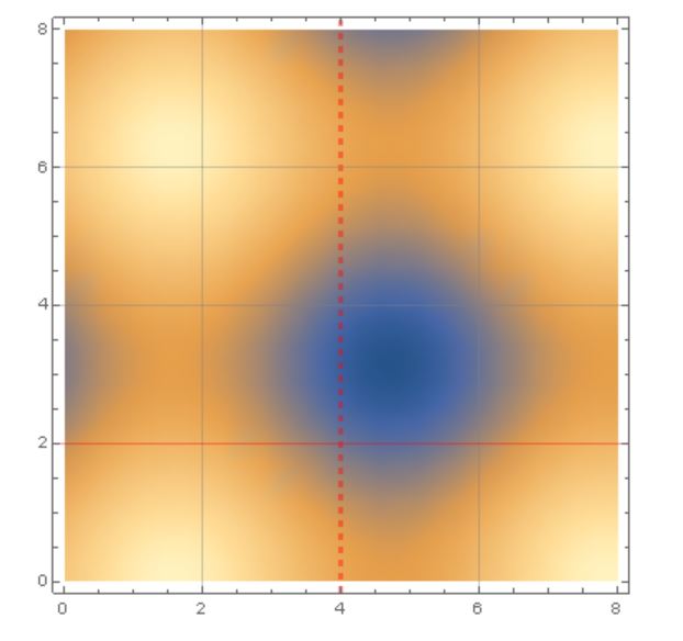
也可以对某一条线进行变化

(*也可以对某一特殊的直线进行变化*)
DensityPlot[
 Sin[x] + Cos[y], {x, 0, 8}, {y, 0, 8},
 GridLines -> {{2, {4, Directive[Red, Dashed, Thickness[.01]]}, 
    6}, {{2, Red}, 4, 6}},
 Method -> {"GridLinesInFront" -> True}
 ]

得到下面的图

看一个线在前面在后面的区别

data = Table[
   Sum[Sin[RandomReal[2]*x] + i/4, {10 i}],
   {i, 1, 4}, {x, 0, 5, 0.5}
   ];

GraphicsRow[
 ListLinePlot[
    data,
    PlotStyle -> 
     Thread[{ColorData[13, "ColorRules"], Thickness[.008]}],
    Method -> {"GridLinesInFront" -> #},
    GridLines -> Automatic,
    GridLinesStyle -> 
     Directive[AbsoluteThickness[2], Opacity[.8], White],
    Background -> Lighter[Gray, .9],
    Axes -> None,
    Frame -> {{True, False}, {True, False}}] & /@ {True, False},
 ImageSize -> 900
 ]
(*线在前面 线在后面*)

得到下面的图

上面就大概把美化讲了一下

2016/8/16

以上，所有

转载于:https://www.cnblogs.com/wmn7q/p/7265574.html