[转载]Bloom filter 以及[转载]中文详解

最新推荐文章于 2022-12-05 20:09:51 发布

weixin_30840253

最新推荐文章于 2022-12-05 20:09:51 发布

阅读量347

点赞数

文章标签：数据结构与算法数据库开发工具

原文链接：http://www.cnblogs.com/roger-mao/archive/2013/05/17/3083216.html

版权

Algorithm description

An example of a Bloom filter, representing the set { x, y, z}. The colored arrows show the positions in the bit array that each set element is mapped to. The element w is not in the set {x, y, z}, because it hashes to one bit-array position containing 0. For this figure, m=18 and k=3.

An empty Bloom filter is a bit array of m bits, all set to 0. There must also be k different hash functions defined, each of which maps or hashes some set element to one of the m array positions with a uniform random distribution.

To add an element, feed it to each of the k hash functions to get k array positions. Set the bits at all these positions to 1.

To query for an element (test whether it is in the set), feed it to each of the k hash functions to get k array positions. If any of the bits at these positions are 0, the element is definitely not in the set – if it were, then all the bits would have been set to 1 when it was inserted. If all are 1, then either the element is in the set, or the bits have by chance been set to 1 during the insertion of other elements, resulting in a false positive. In a simple bloom filter, there is no way to distinguish between the two cases, but more advanced techniques can address this problem.

The requirement of designing k different independent hash functions can be prohibitive for large k. For a good hash function with a wide output, there should be little if any correlation between different bit-fields of such a hash, so this type of hash can be used to generate multiple "different" hash functions by slicing its output into multiple bit fields. Alternatively, one can pass k different initial values (such as 0, 1, ..., k − 1) to a hash function that takes an initial value; or add (or append) these values to the key. For larger m and/or k, independence among the hash functions can be relaxed with negligible increase in false positive rate (Dillinger & Manolios (2004a), Kirsch & Mitzenmacher (2006)). Specifically, Dillinger & Manolios (2004b) show the effectiveness of deriving the k indices using enhanced double hashing or triple hashing, variants of double hashing that are effectively simple random number generators seeded with the two or three hash values.

Removing an element from this simple Bloom filter is impossible because false negatives are not permitted. An element maps to k bits, and although setting any one of those k bits to zero suffices to remove the element, it also results in removing any other elements that happen to map onto that bit. Since there is no way of determining whether any other elements have been added that affect the bits for an element to be removed, clearing any of the bits would introduce the possibility for false negatives.

One-time removal of an element from a Bloom filter can be simulated by having a second Bloom filter that contains items that have been removed. However, false positives in the second filter become false negatives in the composite filter, which may be undesirable. In this approach re-adding a previously removed item is not possible, as one would have to remove it from the "removed" filter.

It is often the case that all the keys are available but are expensive to enumerate (for example, requiring many disk reads). When the false positive rate gets too high, the filter can be regenerated; this should be a relatively rare event.

Space and time advantages

Bloom filter used to speed up answers in a key-value storage system. Values are stored on a disk which has slow access times. Bloom filter decisions are much faster. However some unnecessary disk accesses are made when the filter reports a positive (in order to weed out the false positives). Overall answer speed is better with the Bloom filter than without the Bloom filter. Use of a Bloom filter for this purpose, however, does increase memory usage.

While risking false positives, Bloom filters have a strong space advantage over other data structures for representing sets, such as self-balancing binary search trees, tries, hash tables, or simple arrays or linked lists of the entries. Most of these require storing at least the data items themselves, which can require anywhere from a small number of bits, for small integers, to an arbitrary number of bits, such as for strings (tries are an exception, since they can share storage between elements with equal prefixes). Linked structures incur an additional linear space overhead for pointers. A Bloom filter with 1% error and an optimal value of k, in contrast, requires only about 9.6 bits per element — regardless of the size of the elements. This advantage comes partly from its compactness, inherited from arrays, and partly from its probabilistic nature. If a 1% false-positive rate seems too high, adding about 4.8 bits per element decreases it by ten times.

However, if the number of potential values is small and many of them can be in the set, the Bloom filter is easily surpassed by the deterministic bit array, which requires only one bit for each potential element. Note also that hash tables gain a space and time advantage if they begin ignoring collisions and store only whether each bucket contains an entry; in this case, they have effectively become Bloom filters with k = 1.^[2]

Bloom filters also have the unusual property that the time needed either to add items or to check whether an item is in the set is a fixed constant, O(k), completely independent of the number of items already in the set. No other constant-space set data structure has this property, but the average access time of sparse hash tables can make them faster in practice than some Bloom filters. In a hardware implementation, however, the Bloom filter shines because its k lookups are independent and can be parallelized.

To understand its space efficiency, it is instructive to compare the general Bloom filter with its special case when k = 1. If k = 1, then in order to keep the false positive rate sufficiently low, a small fraction of bits should be set, which means the array must be very large and contain long runs of zeros. The information content of the array relative to its size is low. The generalized Bloom filter (k greater than 1) allows many more bits to be set while still maintaining a low false positive rate; if the parameters (k and m) are chosen well, about half of the bits will be set, and these will be apparently random, minimizing redundancy and maximizing information content.

Probability of false positives

The false positive probability $p$ as a function of number of elements $n$ in the filter and the filter size $m$ . An optimal number of hash functions $k= (m/n) \ln 2$ has been assumed.

Assume that a hash function selects each array position with equal probability. If m is the number of bits in the array, and k is the number of hash functions, then the probability that a certain bit is not set to 1 by a certain hash function during the insertion of an element is then

$1-\frac{1}{m}.$

The probability that it is not set to 1 by any of the hash functions is

$\left(1-\frac{1}{m}\right)^k.$

If we have inserted n elements, the probability that a certain bit is still 0 is

$\left(1-\frac{1}{m}\right)^{kn};$

the probability that it is 1 is therefore

$1-\left(1-\frac{1}{m}\right)^{kn}.$

Now test membership of an element that is not in the set. Each of the k array positions computed by the hash functions is 1 with a probability as above. The probability of all of them being 1, which would cause the algorithm to erroneously claim that the element is in the set, is often given as

$\left(1-\left[1-\frac{1}{m}\right]^{kn}\right)^k \approx \left( 1-e^{-kn/m} \right)^k.$

This is not strictly correct as it assumes independence for the probabilities of each bit being set. However, assuming it is a close approximation we have that the probability of false positives decreases as m (the number of bits in the array) increases, and increases as n (the number of inserted elements) increases. For a given m and n, the value of k (the number of hash functions) that minimizes the probability is

$k = \frac{m}{n} \ln 2,$

which gives

$2^{-k} \approx {0.6185}^{m/n}.$

The required number of bits m, given n (the number of inserted elements) and a desired false positive probability p (and assuming the optimal value of k is used) can be computed by substituting the optimal value of k in the probability expression above:

$p = \left( 1-e^{-(m/n\ln 2) n/m} \right)^{(m/n\ln 2)}$

which can be simplified to:

$\ln p = -\frac{m}{n} \left(\ln 2\right)^2.$

This results in:

$m=-\frac{n\ln p}{(\ln 2)^2}.$

This means that for a given false positive probability p, the length of a Bloom filter m is proportionate to the number of elements being filtered n.^[3] While the above formula is asymptotic (i.e. applicable as m,n → ∞), the agreement with finite values of m,n is also quite good; the false positive probability for a finite bloom filter with m bits, n elements, and k hash functions is at most

$\left( 1-e^{-k(n+0.5)/(m-1)} \right)^k.$

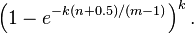
So we can use the asymptotic formula if we pay a penalty for at most half an extra element and at most one fewer bit.^[4]

Approximating the Number of Items in a Bloom Filter

Swamidass & Baldi (2007) showed that the number of items in a bloom filter can be approximated with the following formula,

$X^* = -N \ln \left[ 1 - X / N \right] / k$

where is an estimate of the number of items in the filter, N is length of the filter, k is the number of hash functions per item, and X is the number of bits set to one.

The Union and Intersection of Sets

Bloom filters are a way of compactly representing a set of items. It is common to try and compute the size of the intersection or union between two sets. Bloom filters can be used to approximate the size of the intersection and union of two sets. Swamidass & Baldi (2007) showed that for two bloom filters of length $N$ , their counts, respectively can be estimated as

$A^* = -N \ln \left[ 1 - A / N \right] / k$

and

$B^* = -N \ln \left[ 1 - B / N \right]/k$ .

The size of their union can be estimated as

$A^*\cup B^* = -N \ln \left[ 1 - A \cup B / N \right]/k$ ,

where $A \cup B$ is the number of bits set to one in either of the two bloom filters. And the intersection can be estimated as

$A^*\cap B^* = A^* + B^* - A^*\cup B^*$ ,

Using the three formulas together.

Interesting properties

Unlike sets based on hash tables, any Bloom filter can represent the entire universe of elements. In this case, all bits are 1. Another consequence of this property is that add never fails due to the data structure "filling up." However, the false positive rate increases steadily as elements are added until all bits in the filter are set to 1, so a negative value is never returned. At this point, the Bloom filter completely ceases to differentiate between differing inputs, and is functionally useless.

Union and intersection of Bloom filters with the same size and set of hash functions can be implemented with bitwise OR and AND operations, respectively. The union operation on Bloom filters is lossless in the sense that the resulting Bloom filter is the same as the Bloom filter created from scratch using the union of the two sets. The intersect operation satisfies a weaker property: the false positive probability in the resulting Bloom filter is at most the false-positive probability in one of the constituent Bloom filters, but may be larger than the false positive probability in the Bloom filter created from scratch using the intersection of the two sets.

Some kinds of superimposed code can be seen as a Bloom filter implemented with physical edge-notched cards.

Examples

Google BigTable and Apache Cassandra use Bloom filters to reduce the disk lookups for non-existent rows or columns. Avoiding costly disk lookups considerably increases the performance of a database query operation.^[5]

The Google Chrome web browser uses a Bloom filter to identify malicious URLs. Any URL is first checked against a local Bloom filter and only upon a hit a full check of the URL is performed.^[6]

The Squid Web Proxy Cache uses Bloom filters for cache digests.^[7]

Bitcoin uses Bloom filters to verify payments without running a full network node.^[8]^[9]

The Venti archival storage system uses Bloom filters to detect previously stored data.^[10]

The SPIN model checker uses Bloom filters to track the reachable state space for large verification problems.^[11]

The Cascading analytics framework uses Bloomfilters to speed up asymmetric joins, where one of the joined data sets is significantly larger than the other (often called Bloom join^[12] in the database literature).^[13]

Alternatives

Classic Bloom filters use $1.44\log_2(1/\epsilon)$ bits of space per inserted key, where $\epsilon$ is the false positive rate of the Bloom filter. However, the space that is strictly necessary for any data structure playing the same role as a Bloom filter is only $\log_2(1/\epsilon)$ per key (Pagh, Pagh & Rao 2005). Hence Bloom filters use 44% more space than a hypothetical equivalent optimal data structure. The number of hash functions used to achieve a given false positive rate $\epsilon$ is proportional to $1/\epsilon$ which is not optimal as it has been proved that an optimal data structure would need only a constant number of hash functions independent of the false positive rate.

Stern & Dill (1996) describe a probabilistic structure based on hash tables, hash compaction, which Dillinger & Manolios (2004b) identify as significantly more accurate than a Bloom filter when each is configured optimally. Dillinger and Manolios, however, point out that the reasonable accuracy of any given Bloom filter over a wide range of numbers of additions makes it attractive for probabilistic enumeration of state spaces of unknown size. Hash compaction is, therefore, attractive when the number of additions can be predicted accurately; however, despite being very fast in software, hash compaction is poorly suited for hardware because of worst-case linear access time.

Putze, Sanders & Singler (2007) have studied some variants of Bloom filters that are either faster or use less space than classic Bloom filters. The basic idea of the fast variant is to locate the k hash values associated with each key into one or two blocks having the same size as processor's memory cache blocks (usually 64 bytes). This will presumably improve performance by reducing the number of potential memory cache misses. The proposed variants have however the drawback of using about 32% more space than classic Bloom filters.

The space efficient variant relies on using a single hash function that generates for each key a value in the range $\left[0,n/\varepsilon\right]$ where $\epsilon$ is the requested false positive rate. The sequence of values is then sorted and compressed using Golomb coding (or some other compression technique) to occupy a space close to $n\log_2(1/\epsilon)$ bits. To query the Bloom filter for a given key, it will suffice to check if its corresponding value is stored in the Bloom filter. Decompressing the whole Bloom filter for each query would make this variant totally unusable. To overcome this problem the sequence of values is divided into small blocks of equal size that are compressed separately. At query time only half a block will need to be decompressed on average. Because of decompression overhead, this variant may be slower than classic Bloom filters but this may be compensated by the fact that a single hash function need to be computed.

Another alternative to classic Bloom filter is the one based on space efficient variants of cuckoo hashing. In this case once the hash table is constructed, the keys stored in the hash table are replaced with short signatures of the keys. Those signatures are strings of bits computed using a hash function applied on the keys.

Extensions and applications

Counting filters

Counting filters provide a way to implement a delete operation on a Bloom filter without recreating the filter afresh. In a counting filter the array positions (buckets) are extended from being a single bit to being an n-bit counter. In fact, regular Bloom filters can be considered as counting filters with a bucket size of one bit. Counting filters were introduced by Fan et al. (1998).

The insert operation is extended to increment the value of the buckets and the lookup operation checks that each of the required buckets is non-zero. The delete operation, obviously, then consists of decrementing the value of each of the respective buckets.

Arithmetic overflow of the buckets is a problem and the buckets should be sufficiently large to make this case rare. If it does occur then the increment and decrement operations must leave the bucket set to the maximum possible value in order to retain the properties of a Bloom filter.

The size of counters is usually 3 or 4 bits. Hence counting Bloom filters use 3 to 4 times more space than static Bloom filters. In theory, an optimal data structure equivalent to a counting Bloom filter should not use more space than a static Bloom filter.

Another issue with counting filters is limited scalability. Because the counting Bloom filter table cannot be expanded, the maximal number of keys to be stored simultaneously in the filter must be known in advance. Once the designed capacity of the table is exceeded, the false positive rate will grow rapidly as more keys are inserted.

Bonomi et al. (2006) introduced a data structure based on d-left hashing that is functionally equivalent but uses approximately half as much space as counting Bloom filters. The scalability issue does not occur in this data structure. Once the designed capacity is exceeded, the keys could be reinserted in a new hash table of double size.

The space efficient variant by Putze, Sanders & Singler (2007) could also be used to implement counting filters by supporting insertions and deletions.

Data synchronization

Bloom filters can be used for approximate data synchronization as in Byers et al. (2004). Counting Bloom filters can be used to approximate the number of differences between two sets and this approach is described in Agarwal & Trachtenberg (2006).

Bloomier filters

Chazelle et al. (2004) designed a generalization of Bloom filters that could associate a value with each element that had been inserted, implementing an associative array. Like Bloom filters, these structures achieve a small space overhead by accepting a small probability of false positives. In the case of "Bloomier filters", a false positive is defined as returning a result when the key is not in the map. The map will never return the wrong value for a key that is in the map.

Compact approximators

Boldi & Vigna (2005) proposed a lattice-based generalization of Bloom filters. A compact approximator associates to each key an element of a lattice (the standard Bloom filters being the case of the Boolean two-element lattice). Instead of a bit array, they have an array of lattice elements. When adding a new association between a key and an element of the lattice, they compute the maximum of the current contents of the k array locations associated to the key with the lattice element. When reading the value associated to a key, they compute the minimum of the values found in the k locations associated to the key. The resulting value approximates from above the original value.

Stable Bloom filters

Deng & Rafiei (2006) proposed Stable Bloom filters as a variant of Bloom filters for streaming data. The idea is that since there is no way to store the entire history of a stream (which can be infinite), Stable Bloom filters continuously evict stale information to make room for more recent elements. Since stale information is evicted, the Stable Bloom filter introduces false negatives, which do not appear in traditional bloom filters. The authors show that a tight upper bound of false positive rates is guaranteed, and the method is superior to standard bloom filters in terms of false positive rates and time efficiency when a small space and an acceptable false positive rate are given.

Scalable Bloom filters

Almeida et al. (2007) proposed a variant of Bloom filters that can adapt dynamically to the number of elements stored, while assuring a minimum false positive probability. The technique is based on sequences of standard bloom filters with increasing capacity and tighter false positive probabilities, so as to ensure that a maximum false positive probability can be set beforehand, regardless of the number of elements to be inserted.

Attenuated Bloom filters

An attenuated bloom filter of depth D can be viewed as an array of D normal bloom filters. In the context of service discovery in a network, each node stores regular and attenuated bloom filters locally. The regular or local bloom filter indicates which services are offered by the node itself. The attenuated filter of level i indicates which services can be found on nodes that are i-hops away from the current node. The i-th value is constructed by taking a union of local bloom filters for nodes i-hops away from the node.^[14]

Attenuated Bloom Filter Example

Lets take a small network shown on the graph below as an example. Say we are searching for a service A whose id hashes to bits 0,1, and 3 (pattern 11010). Let n1 node to be the starting point. First, we check whether service A is offered by n1 by checking its local filter. Since the patterns don't match, we check the attenuated bloom filter in order to determine which node should be the next hop. We see that n2 doesn't offer service A but lies on the path to nodes that do. Hence, we move to n2 and repeat the same procedure. We quickly find that n3 offers the service, and hence the destination is located.^[15]

By using attenuated Bloom filters consisting of multiple layers, services at more than one hop distance can be discovered while avoiding saturation of the Bloom filter by attenuating (shifting out) bits set by sources further away.^[14]

Chemical Structure Searching

Bloom filters are commonly used to search large databases of chemicals (see chemical similarity). Each molecule is represented with a bloom filter (called a fingerprint in this field) which stores substructures of the molecule. Commonly, the tanimoto similarity is used to quantify the similarity between molecules' bloom filters.

转自：http://www.cnblogs.com/allensun/archive/2011/02/16/1956532.html

布隆过滤器 (Bloom Filter)是由Burton Howard Bloom于1970年提出，它是一种space efficient的概率型数据结构，用于判断一个元素是否在集合中。在垃圾邮件过滤的黑白名单方法、爬虫(Crawler)的网址判重模块中等等经常被用到。哈希表也能用于判断元素是否在集合中，但是布隆过滤器只需要哈希表的1/8或1/4的空间复杂度就能完成同样的问题。布隆过滤器可以插入元素，但不可以删除已有元素。其中的元素越多，false positive rate(误报率)越大，但是false negative (漏报)是不可能的。

本文将详解布隆过滤器的相关算法和参数设计，在此之前希望大家可以先通过谷歌黑板报的数学之美系列二十一－布隆过滤器（Bloom Filter）来得到些基础知识。

一. 算法描述

一个empty bloom filter是一个有m bits的bit array，每一个bit位都初始化为0。并且定义有k个不同的hash function，每个都以uniform random distribution将元素hash到m个不同位置中的一个。在下面的介绍中n为元素数，m为布隆过滤器或哈希表的slot数，k为布隆过滤器重 hash function数。

为了add一个元素，用k个hash function将它hash得到bloom filter中k个bit位，将这k个bit位置1。

为了query一个元素，即判断它是否在集合中，用k个hash function将它hash得到k个bit位。若这k bits全为1，则此元素在集合中；若其中任一位不为1，则此元素比不在集合中（因为如果在，则在add时已经把对应的k个bits位置为1）。

不允许remove元素，因为那样的话会把相应的k个bits位置为0，而其中很有可能有其他元素对应的位。因此remove会引入false negative，这是绝对不被允许的。

当 k很大时，设计k个独立的hash function是不现实并且困难的。对于一个输出范围很大的hash function（例如MD5产生的128 bits数），如果不同bit位的相关性很小，则可把此输出分割为k份。或者可将k个不同的初始值（例如0,1,2, … ,k-1）结合元素，feed给一个hash function从而产生k个不同的数。

当add的元素过多时，即n/m过大时（n是元素数，m是bloom filter的bits数），会导致false positive过高，此时就需要重新组建filter，但这种情况相对少见。

二. 时间和空间上的优势

当可以承受一些误报时，布隆过滤器比其它表示集合的数据结构有着很大的空间优势。例如self-balance BST, tries, hash table或者array, chain，它们中大多数至少都要存储元素本身，对于小整数需要少量的bits，对于字符串则需要任意多的bits（tries是个例外，因为对于有相同 prefixes的元素可以共享存储空间）；而chain结构还需要为存储指针付出额外的代价。对于一个有1%误报率和一个最优k值的布隆过滤器来说，无论元素的类型及大小，每个元素只需要9.6 bits来存储。这个优点一部分继承自array的紧凑性，一部分来源于它的概率性。如果你认为1%的误报率太高，那么对每个元素每增加4.8 bits，我们就可将误报率降低为原来的1/10。add和query的时间复杂度都为O(k)，与集合中元素的多少无关，这是其他数据结构都不能完成的。

如果可能元素范围不是很大，并且大多数都在集合中，则使用确定性的bit array远远胜过使用布隆过滤器。因为bit array对于每个可能的元素空间上只需要1 bit，add和query的时间复杂度只有O(1)。注意到这样一个哈希表（bit array）只有在忽略collision并且只存储元素是否在其中的二进制信息时，才会获得空间和时间上的优势，而在此情况下，它就有效地称为了k=1 的布隆过滤器。

而当考虑到collision时，对于有m个slot的bit array或者其他哈希表（即k=1的布隆过滤器），如果想要保证1%的误判率，则这个bit array只能存储m/100个元素，因而有大量的空间被浪费，同时也会使得空间复杂度急剧上升，这显然不是space efficient的。解决的方法很简单，使用k>1的布隆过滤器，即k个hash function将每个元素改为对应于k个bits，因为误判度会降低很多，并且如果参数k和m选取得好，一半的m可被置为为1，这充分说明了布隆过滤器的space efficient性。

三. 举例说明

以垃圾邮件过滤中黑白名单为例：现有1亿个email的黑名单，每个都拥有8 bytes的指纹信息，则可能的元素范围为，对于bit array来说是根本不可能的范围，而且元素的数量（即email列表）为，相比于元素范围过于稀疏，而且还没有考虑到哈希表中的collision问题。

若采用哈希表，由于大多数采用open addressing来解决collision，而此时的search时间复杂度为：

即若哈希表半满(n/m = 1/2)，则每次search需要probe 2次，因此在保证效率的情况下哈希表的存储效率最好不超过50%。此时每个元素占8 bytes，总空间为：

若采用Perfect hashing（这里可以采用Perfect hashing是因为主要操作是search/query，而并不是add和remove），虽然保证worst-case也只有一次probe，但是空间利用率更低，一般情况下为50%，worst-case时有不到一半的概率为25%。

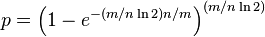
若采用布隆过滤器，取k=8。因为n为1亿，所以总共需要被置位为1，又因为在保证误判率低且k和m选取合适时，空间利用率为50%（后面会解释），所以总空间为：

所需空间比上述哈希结构小得多，并且误判率在万分之一以下。

四. 误判概率的证明和计算

假设布隆过滤器中的hash function满足simple uniform hashing假设：每个元素都等概率地hash到m个slot中的任何一个，与其它元素被hash到哪个slot无关。若m为bit数，则对某一特定 bit位在一个元素由某特定hash function插入时没有被置位为1的概率为：

则k个hash function中没有一个对其置位的概率为：

如果插入了n个元素，但都未将其置位的概率为：

则此位被置位的概率为：

现在考虑query阶段，若对应某个待query元素的k bits全部置位为1，则可判定其在集合中。因此将某元素误判的概率为：

由于，并且当m很大时趋近于0，所以

从上式中可以看出，当m增大或n减小时，都会使得误判率减小，这也符合直觉。

现在计算对于给定的m和n，k为何值时可以使得误判率最低。设误判率为k的函数为：

设，则简化为

，两边取对数

, 两边对k求导

下面求最值

因此，即当时误判率最低，此时误判率为：

可以看出若要使得误判率≤1/2，则：

这说明了若想保持某固定误判率不变，布隆过滤器的bit数m与被add的元素数n应该是线性同步增加的。

五. 设计和应用布隆过滤器的方法

应用时首先要先由用户决定要add的元素数n和希望的误差率P。这也是一个设计完整的布隆过滤器需要用户输入的仅有的两个参数，之后的所有参数将由系统计算，并由此建立布隆过滤器。

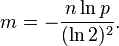
系统首先要计算需要的内存大小m bits:

再由m，n得到hash function的个数：

至此系统所需的参数已经备齐，接下来add n个元素至布隆过滤器中，再进行query。

根据公式，当k最优时：

因此可验证当P=1%时，存储每个元素需要9.6 bits：

而每当想将误判率降低为原来的1/10，则存储每个元素需要增加4.8 bits：

这里需要特别注意的是，9.6 bits/element不仅包含了被置为1的k位，还把包含了没有被置为1的一些位数。此时的

才是每个元素对应的为1的bit位数。

从而使得P(error)最小时，我们注意到：

中的，即

此概率为某bit位在插入n个元素后未被置位的概率。因此，想保持错误率低，布隆过滤器的空间使用率需为50%。

转载于:https://www.cnblogs.com/roger-mao/archive/2013/05/17/3083216.html

weixin_30840253

关注

0
点赞
踩
0

收藏

觉得还不错? 一键收藏
0
评论
[转载]Bloom filter 以及[转载]中文详解

Algorithm descriptionAn example of a Bloom filter, representing the set {x, y, z}. The colored arrows show the positions in the bit array that each set element is mapped to. The element w is...
复制链接

扫一扫