


在tensorflow中自带了tensorboard面板 可以 让tensorflow 训练过程可视化显示
首先我们先看看我们上面的alexnet模型我们怎么添加tensorboard相关的op操作 添加到session回话中,让给该op收集训练过程数据 写入日志,收集汇总起来用来图表可视化显示
官方文档 https://www.tensorflow.org/versions/r0.8/how_tos/summaries_and_tensorboard/index.html

1.tensorflow 网络 可视化,操作,对于每一步op 形成的无向图,我们可以使用tensorflow可视化 ,因为tensorflow默认每一次回话有一个默认的graph对象 graph.ref
所以
summary_writer = tf.train.SummaryWriter('/tmp/tensorflowlogs', graph_def=sess.graph_def)如果我们需要记录 图标训练时候的参数
我们需要 添加相应的op操作,上面的sumary_writer操作是复杂 将来训练时候的op 过程记录到日志里面,便于后面显示graph
因为变量很多,所以可以定义scope范围来管理,节点树一样展开查看,文档上有 很清晰,这里就不解释了,下面介绍介个方法 记录 op 以及 汇总op的方法
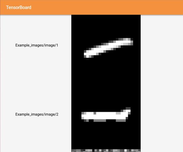
1.4D数据虚拟化 tensorflow 比如CNN每一步生成的特征 ,也就是用图像虚拟化ndarry的特征,比如我们可以看到每一步cnn得到的特征是什么。比如下图 车子 每一步得到的CNN特征 用图像方式虚拟化显示image_summary
images = np.random.randint(256, size=shape).astype(np.uint8)
tf.image_summary("Visualize_image", images) 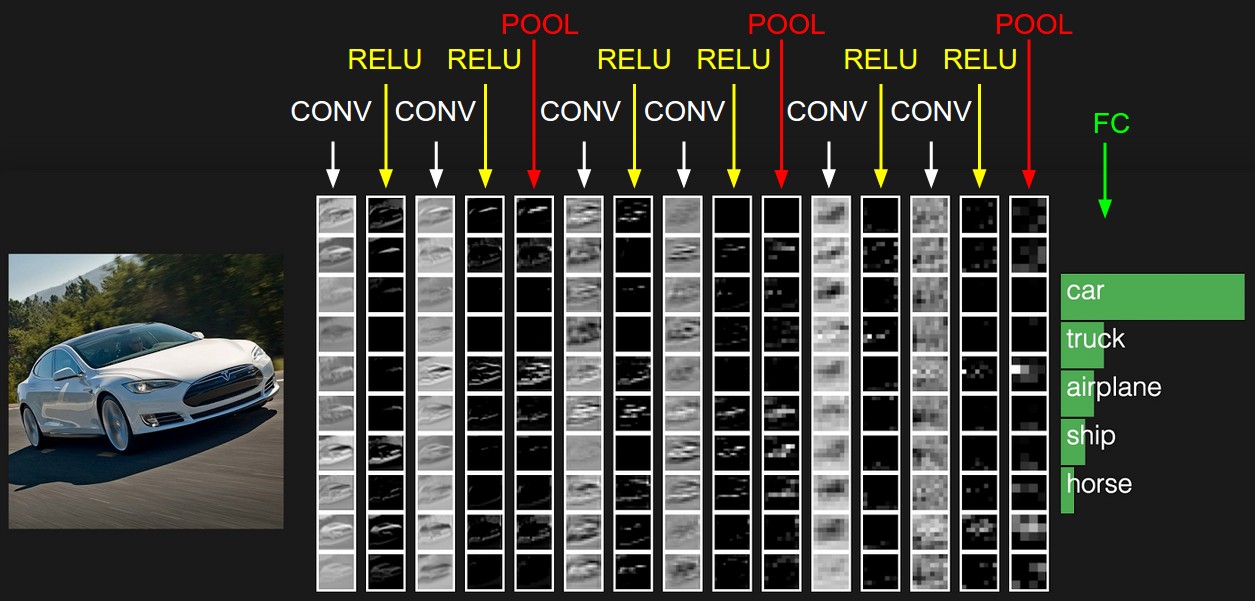
展示的样子大概
2.图标变化方式展示tensorflow数据特征
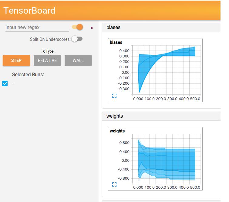
w_hist = tf.histogram_summary("weights", W)
b_hist = tf.histogram_summary("biases", b)
y_hist = tf.histogram_summary("y", y)
大概下面这个样子
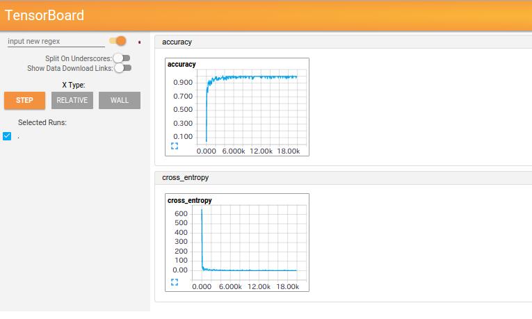
3.以变量批次事件变化的线路图显示表示tensorflow数据
比如下面记录精度的变化曲线图
accuracy_summary = tf.scalar_summary("accuracy", accuracy)展示的样子大概这么个样子
因为我们上面这些op操作各种各样 多个 所以需要有个汇总的op操作
该操作会汇总上面的所有summary
merged = tf.merge_all_summaries()最后在session中执行汇总summary操作op 并使用上面sumarywriter 写入更新到graph 日志中
summary_all = sess.run(merged_summary_op, feed_dict={x: batch_xs, y: batch_ys})
summary_writer.add_summary(summary_all,  i)
现在我们 回到 上面一篇文章的model alexnet中我们添加summary
下面看看我们分别加上了
loss accuracy 的几个summary
import input_data
mnist = input_data.read_data_sets("/tmp/data/", one_hot=True)

import tensorflow as tf

# Parameters
learning_rate = 0.001
training_iters = 200000
batch_size = 64
display_step = 20

# Network Parameters
n_input = 784 # MNIST data input (img shape: 28*28)
n_classes = 10 # MNIST total classes (0-9 digits)
dropout = 0.8 # Dropout, probability to keep units

# tf Graph input
x = tf.placeholder(tf.float32, [None, n_input])
y = tf.placeholder(tf.float32, [None, n_classes])
keep_prob = tf.placeholder(tf.float32) # dropout (keep probability)

# Create custom model
def conv2d(name, l_input, w, b):
    return tf.nn.relu(tf.nn.bias_add(tf.nn.conv2d(l_input, w, strides=[1, 1, 1, 1], padding='SAME'),b), name=name)

def max_pool(name, l_input, k):
    return tf.nn.max_pool(l_input, ksize=[1, k, k, 1], strides=[1, k, k, 1], padding='SAME', name=name)

def norm(name, l_input, lsize=4):
    return tf.nn.lrn(l_input, lsize, bias=1.0, alpha=0.001 / 9.0, beta=0.75, name=name)

def customnet(_X, _weights, _biases, _dropout):
    # Reshape input picture
    _X = tf.reshape(_X, shape=[-1, 28, 28, 1])

    # Convolution Layer
    conv1 = conv2d('conv1', _X, _weights['wc1'], _biases['bc1'])
    # Max Pooling (down-sampling)
    pool1 = max_pool('pool1', conv1, k=2)
    # Apply Normalization
    norm1 = norm('norm1', pool1, lsize=4)
    # Apply Dropout
    norm1 = tf.nn.dropout(norm1, _dropout)
    #conv1 image show
    tf.image_summary("conv1", conv1)
    # Convolution Layer
    conv2 = conv2d('conv2', norm1, _weights['wc2'], _biases['bc2'])
    # Max Pooling (down-sampling)
    pool2 = max_pool('pool2', conv2, k=2)
    # Apply Normalization
    norm2 = norm('norm2', pool2, lsize=4)
    # Apply Dropout
    norm2 = tf.nn.dropout(norm2, _dropout)

    # Convolution Layer
    conv3 = conv2d('conv3', norm2, _weights['wc3'], _biases['bc3'])
    # Max Pooling (down-sampling)
    pool3 = max_pool('pool3', conv3, k=2)
    # Apply Normalization
    norm3 = norm('norm3', pool3, lsize=4)
    # Apply Dropout
    norm3 = tf.nn.dropout(norm3, _dropout)
    #conv4
    conv4 = conv2d('conv4', norm3, _weights['wc4'], _biases['bc4'])
    # Max Pooling (down-sampling)
    pool4 = max_pool('pool4', conv4, k=2)
    # Apply Normalization
    norm4 = norm('norm4', pool4, lsize=4)
    # Apply Dropout
    norm4 = tf.nn.dropout(norm4, _dropout)
    # Fully connected layer
    dense1 = tf.reshape(norm4, [-1, _weights['wd1'].get_shape().as_list()[0]]) # Reshape conv3 output to fit dense layer input
    dense1 = tf.nn.relu(tf.matmul(dense1, _weights['wd1']) + _biases['bd1'], name='fc1') # Relu activation

    dense2 = tf.nn.relu(tf.matmul(dense1, _weights['wd2']) + _biases['bd2'], name='fc2') # Relu activation

    # Output, class prediction
    out = tf.matmul(dense2, _weights['out']) + _biases['out']
    return out

# Store layers weight & bias
weights = {
    'wc1': tf.Variable(tf.random_normal([3, 3, 1, 64])),
    'wc2': tf.Variable(tf.random_normal([3, 3, 64, 128])),
    'wc3': tf.Variable(tf.random_normal([3, 3, 128, 256])),
    'wc4': tf.Variable(tf.random_normal([2, 2, 256, 512])),
    'wd1': tf.Variable(tf.random_normal([2*2*512, 1024])),
    'wd2': tf.Variable(tf.random_normal([1024, 1024])),
    'out': tf.Variable(tf.random_normal([1024, 10]))
}
biases = {
    'bc1': tf.Variable(tf.random_normal([64])),
    'bc2': tf.Variable(tf.random_normal([128])),
    'bc3': tf.Variable(tf.random_normal([256])),
    'bc4': tf.Variable(tf.random_normal([512])),
    'bd1': tf.Variable(tf.random_normal([1024])),
    'bd2': tf.Variable(tf.random_normal([1024])),
    'out': tf.Variable(tf.random_normal([n_classes]))
}

# Construct model
pred = customnet(x, weights, biases, keep_prob)

# Define loss and optimizer
cost = tf.reduce_mean(tf.nn.softmax_cross_entropy_with_logits(pred, y))
optimizer = tf.train.AdamOptimizer(learning_rate=learning_rate).minimize(cost)

# Evaluate model
correct_pred = tf.equal(tf.argmax(pred,1), tf.argmax(y,1))
accuracy = tf.reduce_mean(tf.cast(correct_pred, tf.float32))

# Initializing the variables
init = tf.initialize_all_variables()
#
tf.scalar_summary("loss", cost)
tf.scalar_summary("accuracy", accuracy)
# Merge all summaries to a single operator
merged_summary_op = tf.merge_all_summaries()
# Launch the graph
with tf.Session() as sess:
    sess.run(init)
    summary_writer = tf.train.SummaryWriter('/tmp/logs', graph_def=sess.graph_def)
    step = 1
    # Keep training until reach max iterations
    while step * batch_size < training_iters:
        batch_xs, batch_ys = mnist.train.next_batch(batch_size)
        # Fit training using batch data
        sess.run(optimizer, feed_dict={x: batch_xs, y: batch_ys, keep_prob: dropout})
        if step % display_step == 0:
            # Calculate batch accuracy
            acc = sess.run(accuracy, feed_dict={x: batch_xs, y: batch_ys, keep_prob: 1.})
            # Calculate batch loss
            loss = sess.run(cost, feed_dict={x: batch_xs, y: batch_ys, keep_prob: 1.})
            print "Iter " + str(step*batch_size) + ", Minibatch Loss= " + "{:.6f}".format(loss) + ", Training Accuracy= " + "{:.5f}".format(acc)
            summary_str = sess.run(merged_summary_op, feed_dict={x: batch_xs, y: batch_ys, keep_prob: 1.})
            summary_writer.add_summary(summary_str, step)
        step += 1
    print "Optimization Finished!"
    # Calculate accuracy for 256 mnist test images
    print "Testing Accuracy:", sess.run(accuracy, feed_dict={x: mnist.test.images[:256], y: mnist.test.labels[:256], keep_prob: 1.})
下面我们来启动运行tensorflow tensorborad面板
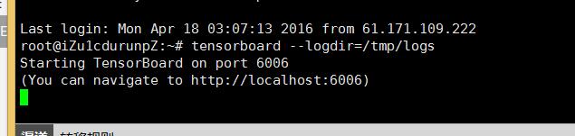
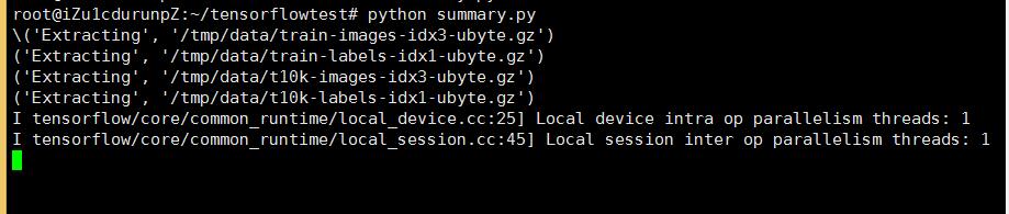
下面打开面板
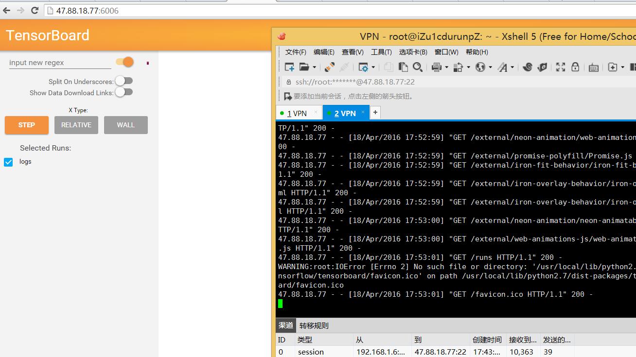
其实大家可能会发现 其实顶部 的四种类型 summary 就是我上面讲的4中类型,如果你添加了相应的summary 会显示相应的区域内

现在才开始 训练 几个的记录 ,后面曲线变化会很明显的 我就不等他运行完截图了。

最后 loss 慢慢 收敛 无变化


 6365
6365

 被折叠的 条评论
为什么被折叠?
被折叠的 条评论
为什么被折叠?
 到【灌水乐园】发言


