神经网络(二):Logistic实践(2)

2019独角兽企业重金招聘Python工程师标准>>>

实现一个sigmoid函数

import numpy as np


def sigmoid(x):
    """
    使用numpy,可支持矢量计算
    sigmod函数，可用于矢量和矩阵
    """
    s = 1.0 / (1 + 1 / np.exp(x))
    return s


x = np.array([1, 2, 3])

print (sigmoid(x))

"""
[ 0.73105858  0.88079708  0.95257413]
"""

计算sigmod函数的导数

def sigmoid_derivative(x):
    s = 1.0 / (1 + 1 / np.exp(x))
    ds = s*(1-s)
    return ds

在训练之前，首先需要读取数据，读取数据的代码如下：

def load_dataset():
    """
    加载数据集
    7.h5为训练集，8.h5为测试集
    """
    train_dataset = h5py.File('/Users/central/PycharmProjects/logistic/7.h5', "r")  # 读取H5文件

    train_set_x_orig = np.array(train_dataset["train_set_x"][:])  # your train set features
    train_set_y_orig = np.array(train_dataset["train_set_y"][:])  # your train set labels

    test_dataset = h5py.File('/Users/central/PycharmProjects/logistic/8.h5', "r")
    test_set_x_orig = np.array(test_dataset["test_set_x"][:])  # your test set features
    test_set_y_orig = np.array(test_dataset["test_set_y"][:])  #

    classes = np.array(test_dataset["list_classes"][:])  # [b'non-cat' b'cat']

    train_set_y_orig = train_set_y_orig.reshape((1, train_set_y_orig.shape[0]))  # 对训练集和测试集标签进行reshape
    test_set_y_orig = test_set_y_orig.reshape((1, test_set_y_orig.shape[0]))

    return train_set_x_orig, train_set_y_orig, test_set_x_orig, test_set_y_orig, classes

数据说明：

对于训练集的标签而言，对于猫，标记为1，否则标记为0。

每一个图像的维度都是(num_px, num_px, 3)，其中，长宽相同，3表示是RGB图像。

train_set_x_orig和test_set_x_orig中，包含_orig是由于我们稍候需要对图像进行预处理，预处理后的变量将会命名为train_set_x和train_set_y。

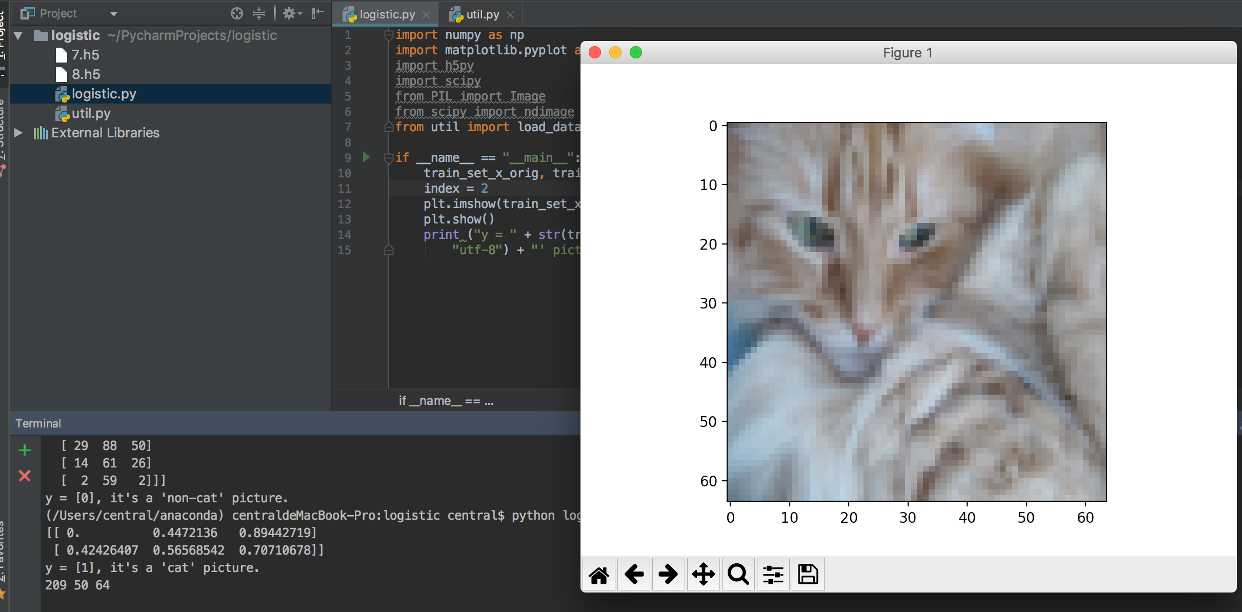
train_set_x_orig中的每一个元素对于这一副图像，我们可以用如下代码将图像显示出来：

if __name__ == "__main__":
    train_set_x_orig, train_set_y, test_set_x_orig, test_set_y, classes = load_dataset();
    index = 2
    plt.imshow(train_set_x_orig[index])
    plt.show()
    print ("y = " + str(train_set_y[:, index]) + ", it's a '" + classes[np.squeeze(train_set_y[:, index])].decode(
        "utf-8") + "' picture.")
"""
y = [1], it's a 'cat' picture.
"""

接下来，我们需要根据图像集来计算出训练集的大小、测试集的大小以及图片的大小：

if __name__ == "__main__":
    train_set_x_orig, train_set_y, test_set_x_orig, test_set_y, classes = load_dataset();
    m_train = train_set_x_orig.shape[0]
    m_test = test_set_x_orig.shape[0]
    num_px = train_set_x_orig.shape[1]
    print(m_train, m_test, num_px)

"""
209 50 64
"""

训练集大小为209,测试集为50，图片的大小为64*64.

接下来，我们需要对将每幅图像转为一个矢量，即矩阵的一列。

最终，整个训练集和测试集将会转为一个矩阵，其中包括num_px*numpy*3行，m_train列。

train_set_x_flatten = train_set_x_orig.reshape(train_set_x_orig.shape[0], -1).T
test_set_x_flatten = test_set_x_orig.reshape(test_set_x_orig.shape[0], -1).T

其中X_flatten = X.reshape(X.shape[0], -1).T可以将一个维度为(a,b,c,d)的矩阵转换为一个维度为(b∗∗c∗∗d, a)的矩阵。

接下来，我们需要对图像值进行归一化。

由于图像的原始值在0到255之间，最简单的方式是直接除以255即可。

train_set_x = train_set_x_flatten/255.
test_set_x = test_set_x_flatten/255.

接下来，我们将按照如下步骤来实现Logistic：

1. 定义模型结构

2. 初始化模型参数

3. 循环

    3.1 前向传播

    3.2 反向传递

    3.3 更新参数

4. 整合成为一个完整的模型

初始化w,b

def init_params(dim):
    #初始化w为dim行，1列的矩阵
    w = np.zeros((dim, 1))
    b = 0
    return w, b

前向传播与反向传播

def propagate(w, b, X, Y):

    #一共有m个训练集
    m = X.shape[1]

    #前向传播
    A = sigmoid(np.dot(w.T, X)+b)
    #代价函数
    cost = -1.0 / m * np.sum(Y * np.log(A) + (1.0 - Y) * np.log(1.0 - A))

    #反向传播
    dw = 1.0 / m * np.dot(X, (A-Y).T)
    db = 1.0 /m * np.sum(A - Y)
    #删除单维数据
    cost = np.squeeze(cost)
    #梯度 
    grads = {
        "dw": dw,
        "db": db
    }
    return cost, grads

更新参数

def upgrade_params(w, b, X, Y, num_iterations, learning_rate, print_cost = False):

    costs = []

    #迭代循环
    for i in range(num_iterations):

        cost, grads = propagate(w, b, X, Y)
        dw = grads["dw"]
        db = grads["db"]

        #更新w,b
        w = w - learning_rate * dw
        b = b - learning_rate * db

        if i%100 ==0:
            costs.append(cost)

        if print_cost and i % 100 == 0:
            print("Cost after iteration %i: %f" % (i, cost))
    params = {"w": w, "b": b}
    grads = {"dw": dw, "db": db}
    
    return params, grads, costs

使用测试集去预测模型：

def predict(w, b, X):
    
    m = X.shape[1]
    Y_predict = np.zeros((1, m))
    w = w.reshape(X.shape[0], 1)
    
    A = sigmoid(np.dot(w.T, X) + b)
    
    for i in range(A.shape[1]):
        if A[0][i] > 0.5
            Y_predict[0][i] = 1
        
        else:
            Y_predict[0][i] = 0
            
    return Y_predict

整合为一个模块:

def model(X_train, Y_train, X_test, Y_test, num_iterations=2000, learning_rate=0.5, print_cost=False):

    #将w,b参数初始化为0
    w, b = init_params(X_train.shape[0])

    #更新优化参数
    parameters, grads, costs = upgrade_params(w, b, X_train, Y_train, num_iterations, learning_rate, print_cost)

    w = parameters["w"]
    b = parameters["b"]
    #预测测试集和训练集
    Y_prediction_test = predict(w, b, X_test)
    Y_prediction_train = predict(w, b, X_train)

    # Print train/test Errors
    print("train accuracy: {} %".format(100 - np.mean(np.abs(Y_prediction_train - Y_train)) * 100))
    print("test accuracy: {} %".format(100 - np.mean(np.abs(Y_prediction_test - Y_test)) * 100))

    d = {"costs": costs,
         "Y_prediction_test": Y_prediction_test,
         "Y_prediction_train": Y_prediction_train,
         "w": w,
         "b": b,
         "learning_rate": learning_rate,
         "num_iterations": num_iterations}

    return d

我们最终来测试一下该模型:

if __name__ == "__main__":
    train_set_x_orig, train_set_y, test_set_x_orig, test_set_y, classes = load_dataset();

    train_set_x_flatten = train_set_x_orig.reshape(train_set_x_orig.shape[0], -1).T
    test_set_x_flatten = test_set_x_orig.reshape(test_set_x_orig.shape[0], -1).T
    #归一化处理图像集
    train_set_x = train_set_x_flatten / 255.
    test_set_x = test_set_x_flatten / 255.
    
    #迭代2000次，学习速率为0.005
    d = model(train_set_x, train_set_y, test_set_x, test_set_y, num_iterations=2000, learning_rate=0.005,
              print_cost=True)


"""
Cost after iteration 0: 0.693147
Cost after iteration 100: 0.584508
Cost after iteration 200: 0.466949
Cost after iteration 300: 0.376007
Cost after iteration 400: 0.331463
Cost after iteration 500: 0.303273
Cost after iteration 600: 0.279880
Cost after iteration 700: 0.260042
Cost after iteration 800: 0.242941
Cost after iteration 900: 0.228004
Cost after iteration 1000: 0.214820
Cost after iteration 1100: 0.203078
Cost after iteration 1200: 0.192544
Cost after iteration 1300: 0.183033
Cost after iteration 1400: 0.174399
Cost after iteration 1500: 0.166521
Cost after iteration 1600: 0.159305
Cost after iteration 1700: 0.152667
Cost after iteration 1800: 0.146542
Cost after iteration 1900: 0.140872
train accuracy: 99.04306220095694 %
test accuracy: 70.0 %

"""

此时，观察打印结果，我们可以发现我们的测试集准确率已经可以达到70.0%。而对于训练集，其准确性达到了99%。这表明了我们的模型有着一定的过拟合，我们会在后续的内容中来解决这一问题。

我们也可以画出代价函数的曲线：

    costs = np.squeeze(d['costs'])
    plt.plot(costs)
    plt.ylabel('cost')
    plt.xlabel('iterations (per hundreds)')
    plt.title("Learning rate =" + str(d["learning_rate"]))
    plt.show()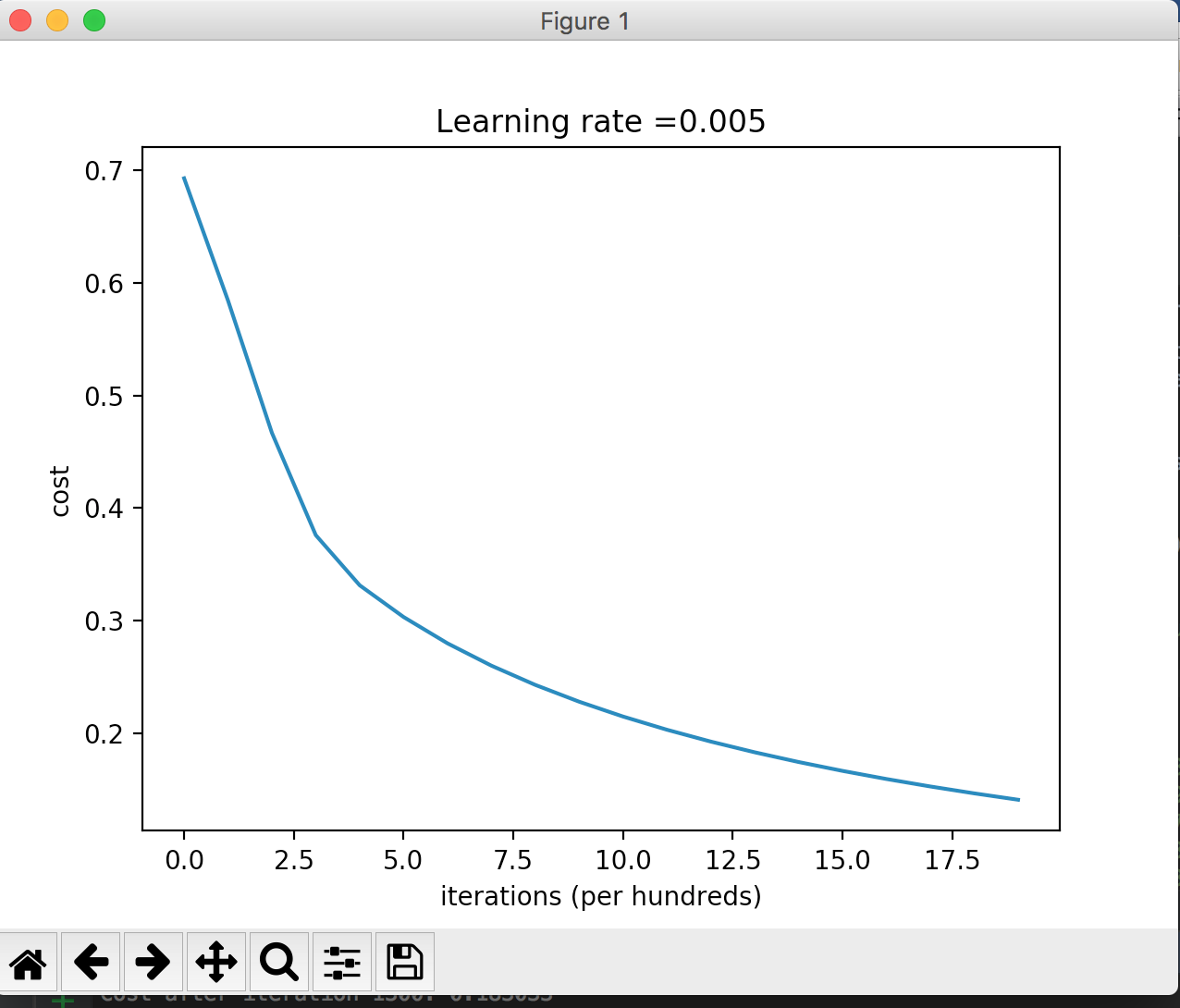

之前的理论课程中，我们已经提及过学习速率对于最终的结果有着较大影响，现在，我们来用实验让大家有一个直观的了解。

train_set_x_orig, train_set_y, test_set_x_orig, test_set_y, classes = load_dataset();

    train_set_x_flatten = train_set_x_orig.reshape(train_set_x_orig.shape[0], -1).T
    test_set_x_flatten = test_set_x_orig.reshape(test_set_x_orig.shape[0], -1).T
    # 归一化处理图像集
    train_set_x = train_set_x_flatten / 255.
    test_set_x = test_set_x_flatten / 255.

    learning_rates = [0.01, 0.001, 0.0001]
    models = {}
    for i in learning_rates:
        print("learning rate is: " + str(i))
        models[str(i)] = model(train_set_x, train_set_y, test_set_x, test_set_y, num_iterations=1500, learning_rate=i,
                               print_cost=False)
        print('\n' + "-------------------------------------------------------" + '\n')

    for i in learning_rates:
        plt.plot(np.squeeze(models[str(i)]["costs"]), label=str(models[str(i)]["learning_rate"]))

    plt.ylabel('cost')
    plt.xlabel('iterations')

    legend = plt.legend(loc='upper center', shadow=True)
    frame = legend.get_frame()
    frame.set_facecolor('0.90')
    plt.show()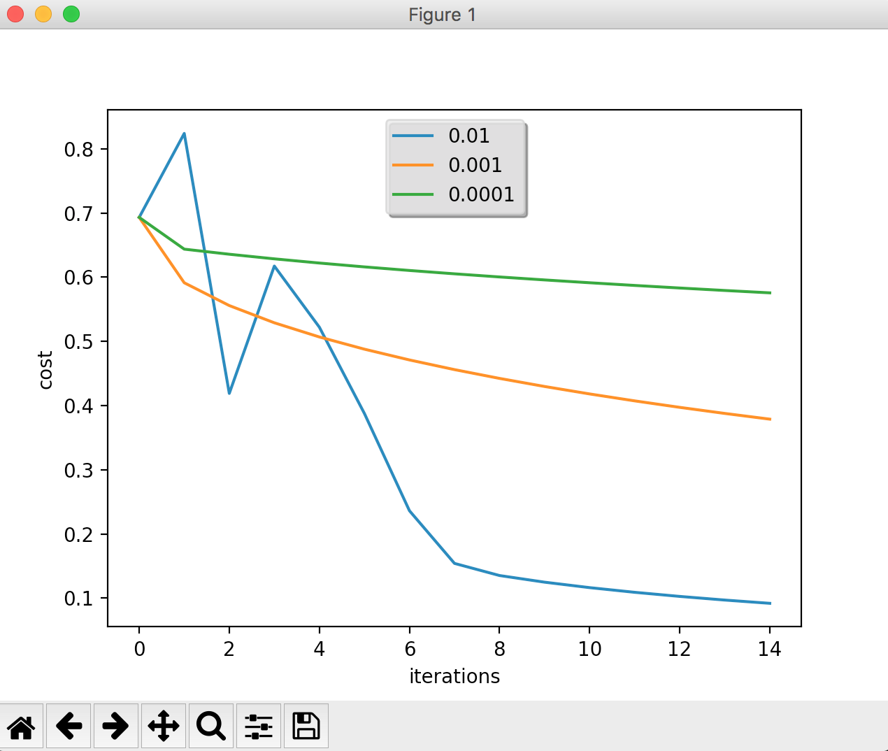

从图中结果反映出不同的学习速率会导致不同的预测结果。较小的学习速度收敛速度较慢，而过大的学习速度可能导致震荡或无法收敛。

如果想用自己的图像做测试，可已使用以下代码：

    my_image = "cat2.jpg"  # change this to the name of your image file
    ## END CODE HERE ##

    # We preprocess the image to fit your algorithm.

    train_set_x_orig, train_set_y, test_set_x_orig, test_set_y, classes = load_dataset();

    train_set_x_flatten = train_set_x_orig.reshape(train_set_x_orig.shape[0], -1).T
    test_set_x_flatten = test_set_x_orig.reshape(test_set_x_orig.shape[0], -1).T
    # 归一化处理图像集
    train_set_x = train_set_x_flatten / 255.
    test_set_x = test_set_x_flatten / 255.
    num_px= 64;

    fname = "picture/" + my_image
    image = np.array(ndimage.imread(fname, flatten=False))  # 读取图片

    my_image = scipy.misc.imresize(image, size=(num_px, num_px)).reshape((1, num_px * num_px * 3)).T  # 放缩图像

    d = model(train_set_x, train_set_y, test_set_x, test_set_y, num_iterations=2000, learning_rate=0.005,
              print_cost=True)

    my_predicted_image = predict(d["w"], d["b"], my_image)  # 预测

    plt.imshow(image)
    print("y = " + str(np.squeeze(my_predicted_image)) + ", your algorithm predicts a \"" + classes[
        int(np.squeeze(my_predicted_image)),].decode("utf-8") + "\" picture.")

注：

之前我的训练样本都是在64*64的样本进行测试，所以使用自己的测试图片时，如果图像像素过大，可能出现预期结果很差的现象，所以我们在测试时可以选择图像像素较小的进行测试。

关于基础算法部分，可以参考:https://my.oschina.net/CentralD/blog/1541585

转载于:https://my.oschina.net/CentralD/blog/1551033