Chi-squared tests

2019独角兽企业重金招聘Python工程师标准>>>

1: Observed And Expected Frequencies

In this mission, we'll be learning about the chi-squared test for categorical data. This test enables us to determine the statistical significance of observing a set of categorical values.

We'll be working with data on US income and demographics throughout this mission. Here are the first few rows of the data, in csv format:

 

age,workclass,fnlwgt,education,education_num,marital_status,occupation,relationship,race,sex,capital_gain,capital_loss,hours_per_week,native_country,high_income

39, State-gov, 77516, Bachelors, 13, Never-married, Adm-clerical, Not-in-family, White, Male, 2174, 0, 40, United-States, <=50K

50, Self-emp-not-inc, 83311, Bachelors, 13, Married-civ-spouse, Exec-managerial, Husband, White, Male, 0, 0, 13, United-States, <=50K

38, Private, 215646, HS-grad, 9, Divorced, Handlers-cleaners, Not-in-family, White, Male, 0, 0, 40, United-States, <=50K

Each row represents a single person who was counted in the 1990 US Census, and contains information about their income and demograpics. Here are some of the relevant columns:

• age -- how old the person is
• workclass -- the type of sector the person is employed in.
• race -- the race of the person.
• sex -- the gender of the person, either Male or Female.

The entire dataset has 32561 rows, and is a sample of the full Census. Of the rows, 10771 are Female, and 21790 are Male. These numbers look a bit off, because the full Census shows that the US is about 50% Male and 50% Female. So our expected values for number of Males and Females would be 16280.5 each.

Here's a diagram:

MaleFemaleTotalObserved217901077132561Expected16280.516280.532561

We know that something looks off, but we don't quite know how to quantify how different the observed and expected values are. We also don't have any way to determine if there's a statistically significant difference between the two groups, and if we need to investigate further.

This is where a chi-squared test can help. The chi-squared test enables us to quantify the difference between sets of observed and expected categorical values.

2: Calculating Differences

Once way that we can determine the differences between observed and expected values is to compute simple proportional differences.

Let's say an expected value is 1000, and the observed value is 1100. We can compute the proportional difference with:

(observed−expected)expected=(1100−1000)1000=.1(observed−expected)expected=(1100−1000)1000=.1

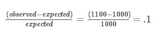
So there's a .1, or 10%, difference between our observed and expected values.

Instructions

In the last screen, our observed values were 10771 Females, and 21790Males. Our expected values were16280.5 Females and 16280.5Males.

• Compute the proportional difference in number of observedFemales vs number of expectedFemales. Assign the result tofemale_diff.
• Compute the proportional difference in number of observedMales vs number of expectedMales. Assign the result tomale_diff\

female_diff=(10771-16280.5)/16280.5
male_diff=(21790-16280.5)/16280.5

 

3: Updating The Formula

In the last screen, we got -0.338 for the Female difference, and 0.338 for the Male difference. These are great for finding individual differences for each category, but since both values add up to 0, they don't give us a meaningful measure of how our overall observed counts deviate from the expected counts.

You may recall this diagram from earlier:

MaleFemaleTotalObserved217901077132561Expected16280.516280.532561

No matter what numbers you plug in for observed Male or Female counts, the differences between observed and expected will always add to 0, because the total observed count for Male and Female items always comes out to 32561. If the observed count ofFemales is high, the count of Males has to be low to compensate, and vice versa.

What we really want to find is one number that can tell us how much all of our observed counts deviate from all of their expected counterparts. This will let us figure out if our difference in counts is statistically significant. We can get one step closer to this by squaring the top term in our difference formula:

(observed−expected)2expected=(1100−1000)21000=10(observed−expected)2expected=(1100−1000)21000=10

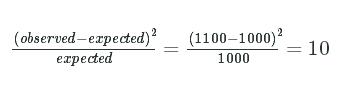
Squaring the difference will ensure that all the differences don't sum to zero (you can't have negative squares), giving us a non-zero number we can use to assess statistical significance.

We can calculate χ2χ2, the chi-squared value, by adding up all of the squared differences between observed and expected values.

Instructions

In the last screen, our observed values were 10771 Females, and 21790Males. Our expected values were16280.5 Females and 16280.5Males.

• Compute the difference in number of observed Females vs number of expected Femalesusing the updated technique. Assign the result tofemale_diff.
• Compute the difference in number of observed Males vs number of expected Males using the updated technique. Assign the result to male_diff.
• Add male_diff andfemale_diff together and assign to the variablegender_chisq.

 

female_diff=(10771-16280.5)**2/16280.5
male_diff=(21790-16280.5)**2/16280.5
gender_chisq=female_diff+male_diff

 

 

4: Generating A Distribution

Now that we have a chi-squared value for our observed and expected gender counts, we need a way to figure out what the chi-squared value represents. We can translate a chi-squared value into a statistical significance value using a chi-squared sampling distribution. If you recall, we covered statistical significance and p-values in the last mission. A p-value allows us to determine whether the difference between two values is due to chance, or due to an underlying difference.

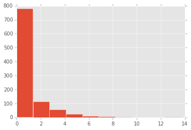
We can generate a chi-squared sampling distribution using our expected probabilities. If we repeatedly generate random samples that contain 32561 samples, and graph the chi-squared value of each sample, we'll be able to generate a distribution. Here's a rough algorithm:

• Randomly generate 32561 numbers that range from 0-1.
• Based on the expected probabilities, assign Male or Female to each number.
• Compute the observed frequences of Male and Female.
• Compute the chi-squared value and save it.
• Repeat several times.
• Create a histogram of all the chi-squared values.

By comparing our chi-squared value to the distribution, and seeing what percentage of the distribution is greater than our value, we'll get a p-value. For instance, if 5% of the values in the distribution are greater than our chi-squared value, the p-value is .05.

Instructions

Inside a for loop that repeats 1000times:

• Use the numpy.random.randomfunction to generate 32561numbers between 0.0 and 1.0.

• Pass (32561,) into thenumpy.random.random function to get a vector with 32561elements.

  • For each of the numbers, if it is less than .5, replace it with 0, otherwise replace it with 1.
  • Count up how many times0 occurs (Malefrequency), and how many times 1 occurs (Femalefrequency).
  • Use the expected frequencies from earlier to compute the chi-squared value.
    • Computemale_diff by subtracting the expected Male count from the observedMale count, squaring it, and dividing by the expected Malecount.
    • Computefemale_diff by subtracting the expected Femalecount from the observed Femalecount, squaring it, and dividing by the expected Femalecount.
    • Add up male_diffand female_diff to get the chi-squared vlaue.

• Append the chi-squared value tochi_squared_values.

• Create a histogram withchi_squared_values using theplt.hist method.

chi_squared_values = []
from numpy.random import random
import matplotlib.pyplot as plt

for i in range(1000):
    sequence=random((32561,))
    sequence[sequence<.5]=0
    sequence[sequence>=.5]=1
    male_count=len(sequence[sequence==0])
    female_count=len(sequence[sequence==1])
    male_diff=(male_count-16280.5)**2/16280.5 
    female_diff=(female_count-16280.5)**2/16280.5
    chi_squared=male_diff+female_diff
    chi_squared_values.append(chi_squared)
plt.hist(chi_squared_values)

 

5: Statistical Significance

In the last screen, our calculated chi-squared value is greater than all the values in the distribution, so our p-value is 0, indicating that our result is statistically significant. You may recall from the last mission that .05 is the typical threshold for statistical significance, and anything below it is considered significant.

A significant value indicates that something is different between the observed and expected values, but it doesn't indicate what is different.

Now that we have a chi-squared sampling distribution, we can compare the chi-squared value we calculated for our data to it to see if our result is statistically significant. The chi-squared value we calculated was 3728.95. The highest value in the chi-squared sampling distribution was about 12. This means that our chi-squared value is higher than 100% of all the values in the sampling distribution, so we get a p-value of 0. This means that there is a 0% chance that we could get such a result randomly.

This would indicate that we need to investigate our data collection techniques more closely to figure out why such a result occurred.

Because a chi-squared value has no sign (all chi-squared values are positive), it doesn't tell us anything about the direction of the statistical significance. If we had 10771 Females, and 21790 Males, or 10771 Males, and 21790 Females, we'd get the same chi-squared value. It's important to look at the data and see how the data is unbalanced after calculating a chi-squared value and getting a significant result.

6: Smaller Samples

One interesting thing about chi-squared values is that they get smaller as the sample size decreases. For example, with our Male andFemale example, let's say we only have 100 rows, but the same observed and expected proportions:

MaleFemaleTotalObserved66.9233.08100Expected5050100

We can compute the chi-squared value for this:

(observedM−expectedM)2expectedM+(observedF−expectedF)2expectedF=(66.92−50)250+(33−50)250=5.726+5.726=11.4522(observedM−expectedM)2expectedM+(observedF−expectedF)2expectedF=(66.92−50)250+(33−50)250=5.726+5.726=11.4522

32561 (our original number of rows) divided by 100 (our new number of rows) is 325.61. If we multiply 11.4522 by 325.61, we get3728.95, which is the exact same chi-squared value that we got two screens ago.

So as sample size changes, the chi-squared value changes proportionally.

Instructions

Let's say our observed values are107.71 Females, and 217.90 Males. Our expected values are 162.805Females and 162.805 Males.

• Compute the difference in number of observed Females vs number of expected Femalesusing the new formula. Assign the result to female_diff.
• Compute the difference in number of observed Males vs number of expected Males using the new formula. Assign the result to male_diff.
• Add male_diff andfemale_diff together and assign to the variablegender_chisq.

 

female_diff=(107.71-162.805)**2/162.805
male_diff=(217.90-162.805)**2/162.805
gender_chisq=female_diff+male_diff

 

7: Sampling Distribution Equality

As sample sizes get larger, seeing large deviations from the expected probabilities gets less and less likely. For example, if you're flipping a coin 10 times, you wouldn't be surprised to see this:

HeadsTailsTotalObserved8210Expected5510

This is a fairly skewed result, but in a small sample size, random chance can create effects like this. It would be very surprising to see this after flipping a coin 1000 times, though:

HeadsTailsTotalObserved8002001000Expected5005001000

A result like this would probably make you check the coin to see if it's a trick coin or weighted improperly.

The chi-squared value follows the same principle. Chi-squared values for the same sized effect increase as sample size increases, but the chance of getting a high chi-squared value decreases as the sample gets larger.

These two effects offset each other, and a chi-squared sampling distribution constructed when sampling 200 items for each iteration will look identical to one sampling 1000 items.

This enables us to easily compare any chi-squared value to a master sampling distribution to determine statistical significance, no matter what sample size the chi-squared value was created with.

Instructions

Inside a for loop that repeats 1000times:

• Use the numpy.random.randomfunction to generate 300numbers between 0.0 and 1.0.
• Pass (300,) into thenumpy.random.random function to get a vector with 300elements.
  • For each of the numbers, if it is less than .5, replace it with 0, otherwise replace it with 1.
  • Count up how many times0 occurs (Malefrequency), and how many times 1 occurs (Femalefrequency).
  • Use the expected frequencies from earlier to compute the chi-squared value.
    • Computemale_diff by subtracting the expected Male count (150) from the observed Malecount, squaring it, and dividing by the expected Malecount.
    • Computefemale_diff by subtracting the expected Femalecount (150) from the observed Femalecount, squaring it, and dividing by the expected Femalecount.
    • Add up male_diffand female_diff to get the chi-squared vlaue.
  • Append the chi-squared value tochi_squared_values.
• Create a histogram withchi_squared_values using theplt.hist method.
• This plot should look identical to the one you generated earlier.

chi_squared_values = []
from numpy.random import random
import matplotlib.pyplot as plt

for i in range(1000):
    sequence = random((300,))
    sequence[sequence < .5] = 0
    sequence[sequence >= .5] = 1
    male_count = len(sequence[sequence == 0])
    female_count = len(sequence[sequence == 1])
    male_diff = (male_count - 150) ** 2 / 150
    female_diff = (female_count - 150) ** 2 / 150
    chi_squared = male_diff + female_diff
    chi_squared_values.append(chi_squared)

plt.hist(chi_squared_values)

 

8: Degrees Of Freedom

When we were computing the chi-squared value earlier, we were working with 2 values that could be vary, the number of Males and the number of Females. But actually, only 1 of the values could vary. Since we already know the total number of values, 32561, if we set one of the values, the other has to be the difference between 32561 and the value we set.

The diagram from earlier might clarify this:

MaleFemaleTotalObserved217901077132561Expected16280.516280.532561

If we set a count for Male or Female, we know what the other value has to be, because they both need to add up to 32561.

A degree of freedom is the number of values that can vary without the other values being "locked in". In the case of our two categories, there is actually only one degree of freedom. Degrees of freedom are an important statistical concept that will come up repeatedly, both in this mission and after.

9: Increasing Degrees Of Freedom

So far, we've only calculated chi-squared values for 2 categories and 1 degree of freedom. We can actually work with any number of categories, and any number of degrees of freedom. We can accomplish this using largely the same formula we've been using, but we will need to generate new sampling distributions for each number of degrees of freedom.

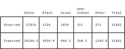
If we look at the race column of the income data, the possible values are White, Black, Asian-Pac-Islander, Amer-Indian-Eskimo, and Other.

We can get our expected proportions straight from the full 1990 US Census:

• White -- 80.3%
• Black -- 12.1%
• Asian-Pac-Islander -- 2.9%
• Amer-Indian-Eskimo -- .8%
• Other -- 3.9%

Here's a table showing expected and actual values for our income dataset:

It looks like there's a discrepancy between the White and Other counts, but let's dig in a bit more and calculate the chi-squared value.

Instructions

• For each category (White,Black, Asian-Pac-Islander,Amer-Indian-Eskimo, andOther):
  • compute the difference between the expected and observed counts,
  • square the difference,
  • divide by the expected value,
  • append each result torace_chisq.

diffs=[]
observed=[27816, 3124, 1039, 311, 271]
expected=[26146.5, 3939.9, 944.3, 260.5, 1269.8]

for i,obs in enumerate(observed):
    exp=expected[i]
    diff=(obs-exp)**2/exp
    diffs.append(diff)
   
race_chisq=sum(diffs)

10: Using SciPy

Rather than constructing another chi-squared sampling distribution for 4 degrees of freedom, we can use a function from the SciPylibrary to do it more quickly.

The scipy.stats.chisquare function takes in an array of observed frequences, and an array of expected frequencies, and returns a tuple containing both the chi-squared value and the matching p-value that we can use to check for statistical significance.

Here's a usage example:

import numpy as np

from scipy.stats import chisquare

​

observed = np.array([5, 10, 15])

expected = np.array([7, 11, 12])

chisquare_value, pvalue = chisquare(observed, expected)

The scipy.stats.chisquare function returns a list, so we can assign each item in the list to a separate variable using 2 variable names separated with a comma, like you see above.

Instructions

• Use the scipy.stats.chisquarefunction to calculate the p-value for the following table

 

• Assign the result torace_pvalue.

import numpy as np
from scipy.stats import chisquare
observed=np.array([27816, 3124, 1039, 311, 271])
expected=np.array([26146.5, 3939.9, 944.3, 260.5, 1269.8])
chisquare_value,race_pvalue=chisquare(observed,expected)

11: Next Steps

In this mission, we introduced the chi-squared test, and showed how to use it to tell if observed and expected categorical frequency data differs significantly. In the next mission, we'll explore how to determine significance in the case of multiple categories.

 

 

 

 

 

 

 

 

转载于:https://my.oschina.net/Bettyty/blog/750352