Machine Learning Project Walkthrough: Making Predictions

2019独角兽企业重金招聘Python工程师标准>>>

1: Recap
We spent the last 2 missions cleaning and preparing a dataset that contains data on loans made to members of Lending Club. Our eventual goal is to generate features from the data, which can feed into a machine learning algorithm. The algorithm will make predictions about whether or not a loan will be paid off on time, which is contained in the loan_status column of the clean dataset.

As we prepared the data, we removed columns that had data leakage issues, contained redundant information, or required additional processing to turn into useful features. We cleaned features that had formatting issues, and converted categorical columns to dummy variables.

In the last mission, we noticed that there's a class imbalance in our target column, loan_status. There are about 6 times as many loans that were paid off on time (positive case, label of 1) than those that weren't (negative case, label of 0). Imbalances can cause issues with many machine learning algorithms, where they appear to have high accuracy, but actually aren't learning from the training data. Because of its potential to cause issues, we need to keep the class imbalance in mind as we build machine learning models.

After all of our data cleaning in the past two missions, we ended up with the csv file called cleaned_loans_2007.csv. Let's read this file into a Dataframe and view a summary of the work we did.

Instructions
Read cleaned_loans_2007.csv into a Dataframe named loans.
Use the info() method and the print function to display a summary of the dataset.

import pandas as pd
loans = pd.read_csv("cleaned_loans_2007.csv")
print(loans.info())

2: Picking An Error Metric

Before we dive into predicting loan_status with machine learning, let's go back to our first steps when we started cleaning the Lending Club dataset. You may recall the original question we wanted to answer:

• Can we build a machine learning model that can accurately predict if a borrower will pay off their loan on time or not?

We established that this is a binary classification problem in the first mission of this course, and we converted the loan_status column to0s and 1s as a result. Before diving in and selecting an algorithm to apply to the data, we should select an error metric.

An error metric will help us figure out when our model is performing well, and when it's performing poorly. To tie error metrics all the way back to the original question we wanted to answer, let's say we're using a machine learning model to predict whether or not we should fund a loan on the Lending Club platform. Our objective in this is to make money -- we want to fund enough loans that are paid off on time to offset our losses from loans that aren't paid off. An error metric will help us determine if our algorithm will make us money or lose us money.

In this case, we're primarily concerned with false positives and false negatives. Both of these are different types of misclassifications. With a false positive, we predict that a loan will be paid off on time, but it actually isn't. This costs us money, since we fund loans that lose us money. With a false negative, we predict that a loan won't be paid off on time, but it actually would be paid off on time. This loses us potential money, since we didn't fund a loan that actually would have been paid off.

Here's a diagram to simplify the concepts:

loan_statuspredictionerrortypeactual01FalsePositive11Truepositive00Truenegative10FalseNegative

In the loan_status and prediction columns, a 0 means that the loan wouldn't be paid off on time, and a 1 means that it would.

Since we're viewing this problem from the standpoint of a conservative investor, we need to treat false positives differently than false negatives. A conservative investor would want to minimize risk, and avoid false positives as much as possible. They'd be more okay with missing out on opportunities (false negatives) than they would be with funding a risky loan (false positives).

Let's calculate false positives and true positives in Python. We can use multiple conditionals, separated by a & to select items in a NumPy array that meet certain conditions. For instance, if we had an array called predictions, we could select items in predictions that equal1 and where items in loans["loan_status"] in the same position also equal 1 using this:

 

filter = (predictions == 1) & (loans["loan_status"] == 1)

predictions[tp_filter]

The above code will give us all the items in predictions that are true positives -- where we predicted that the loan would be paid off on time, and it was actually paid off on time. By using the len function to find the number of items, we can find the number of true positives.

Using the diagram above as a reference, it's possible to compute the other 3 quantities we mentioned -- false positives, true negatives, and false negatives.

We've generated some predictions automatically, and they are stored in a NumPy array called predictions.

Instructions

• Find the number of true negatives.
  • Find the number of items where predictions is 0, and the corresponding entry inloans["loan_status"] is also 0.
  • Assign the result to tn.
• Find the number of true positives.
  • Find the number of items where predictions is 1, and the corresponding entry inloans["loan_status"] is also 1.
  • Assign the result to tp.
• Find the number of false negatives.
  • Find the number of items where predictions is 0, and the corresponding entry inloans["loan_status"] is1.
  • Assign the result to fn.
• Find the number of false positives.
  • Find the number of items where predictions is 1, and the corresponding entry inloans["loan_status"] is0.
  • Assign the result to fp.

import pandas as pd
# False positives.
fp_filter = (predictions == 1) & (loans["loan_status"] == 0)
fp = len(predictions[fp_filter])

# True positives.
tp_filter = (predictions == 1) & (loans["loan_status"] == 1)
tp = len(predictions[tp_filter])

# False negatives.
fn_filter = (predictions == 0) & (loans["loan_status"] == 1)
fn = len(predictions[fn_filter])

# True negatives
tn_filter = (predictions == 0) & (loans["loan_status"] == 0)
tn = len(predictions[tn_filter])

3: Class Imbalance

We mentioned earlier that there is a significant class imbalance in the loan_status column. There are 6 times as many loans that were paid off on time (1), than loans that weren't paid off on time (0). This causes a major issue when we use accuracy as a metric. This is because due to the class imbalance, a classifier can predict 1 for every row, and still have high accuracy. Here's a diagram that illustrates the concept:

loan_statuspredictionactual01111111111111

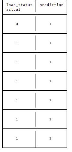
In the above diagram, our predictions are 85.7% accurate -- we've correctly identified loan_status in 85.7% of cases. However, we've done this by predicting 1 for every row. What this means is that we'll actually lose money. Let's say we loan out 1000 dollars on average to each borrower. Each borrower pays us 10% interest back. So we make a projected profit of 100 dollars on each loan. In the above diagram, we'd actually lose money:

loan_statuspredictionprofit/lossactual01-1000111001110011100111001110011100

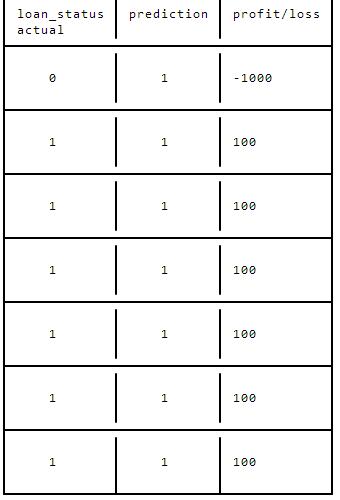
As you can see, we made 600 dollars in interest from the borrowers that paid us back, but we lost 1000 dollars on the one borrower who never paid us back, so we actually ended up losing 400 dollars overall, even though our model is technically accurate.

This is why it's important to always be aware of imbalanced classes in machine learning models, and to adjust your error metric accordingly. In this case, we don't want to use accuracy, and should instead use metrics that tell us the number of false positives and false negatives.

This means that we should optimize for:

• high recall (true positive rate)
• low fall-out (false positive rate)

We can calculate false positive rate and true positive rate, using the numbers of true positives, true negatives, false negatives, and false positives.

False positive rate is the number of false positives divided by the number of false positives plus the number of true negatives. This divides all the cases where we thought a loan would be paid off but it wasn't by all the loans that weren't paid off:

 

fpr = fp / (fp + tn)

True positive rate is the number of true positives divided by the number of true positives plus the number of false negatives. This divides all the cases where we thought a loan would be paid off and it was by all the loans that were paid off:

 

tpr = tp / (tp + fn)

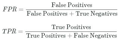
We can write these out as mathematical formulas as well:

FPR=False PositivesFalse Positives+True NegativesFPR=False PositivesFalse Positives+True Negatives

TPR=True PositivesTrue Positives+False NegativesTPR=True PositivesTrue Positives+False Negatives

Simple english ways to think of each term are:

• False Positive Rate -- "what percentage of my 1 predictions are incorrect?"
  • In this case, "what percentage of the loans that I fund would not be repaid?"
• True Positive Rate -- "what percentage of all the possible 1 predictions am I making?"
  • In this case, "what percentage of loans that could be funded would I fund?"

Generally, if we want to reduce false positive rate, true positive rate will also go down. This is because if we want to reduce the risk of false positives, we wouldn't think about funding riskier loans in the first place.

Instructions

• Compute the false positive rate for predictions.
  • Compute the number of false positives, then dived by the number of false positives plus the number of true negatives.
  • Assign to fpr.
• Compute the true positive rate forpredictions.
  • Compute the number of true positives, then dived by the number of true positives plus the number of false negatives.
  • Assign to tpr.
• Print out fpr and tpr to verify.

import pandas as pd
import numpy

# Predict that all loans will be paid off on time.
predictions = pd.Series(numpy.ones(loans.shape[0]))
# False positives.
fp_filter = (predictions == 1) & (loans["loan_status"] == 0)
fp = len(predictions[fp_filter])

# True positives.
tp_filter = (predictions == 1) & (loans["loan_status"] == 1)
tp = len(predictions[tp_filter])

# False negatives.
fn_filter = (predictions == 0) & (loans["loan_status"] == 1)
fn = len(predictions[fn_filter])

# True negatives
tn_filter = (predictions == 0) & (loans["loan_status"] == 0)
tn = len(predictions[tn_filter])

# Rates
tpr = tp / (tp + fn)
fpr = fp / (fp + tn)

print(tpr)
print(fpr)

 

4: Logistic Regression

In the last screen, you may have noticed that both fpr and tpr were 1. This is because we predicted 1 for each row. This means that we correctly identified all of the good loans (true positive rate), but we also incorrectly identified all of the bad loans (false positive rate). Now that we've setup error metrics, we can move on to making predictions using a machine learning algorithm.

As we saw in the first screen of the mission, our cleaned dataset contains 41 columns, all of which are either the int64 or the float64data type. There aren't any null values in any of the columns. This means that we can now apply any machine learning algorithm to our dataset. Most algorithms can't deal with non-numeric or missing values, which is why we had to do so much data cleaning.

In order to fit the machine learning models, we'll use the Scikit-learn library. Although we've built our own implementations of algorithms in earlier missions, it's easier and faster to use algorithms that someone else has already written and tuned for high performance.

A good first algorithm to apply to binary classification problems is logistic regression, for the following reasons:

• it's quick to train and we can iterate more quickly,
• it's less prone to overfitting than more complex models like decision trees,
• it's easy to interpret.

Instructions

• Create a Dataframe namedfeatures that contains just the feature columns.
  • Remove the loan_statuscolumn.
• Create a Series named targetthat contains just the target column (loan_status).
• Use the fit method of lr to fit a logistic regression to featuresand target.
• Use the predict method of lr to make predictions on features. Assign the predictions topredictions.

 

from sklearn.linear_model import LogisticRegression
lr = LogisticRegression()
cols = loans.columns
train_cols = cols.drop("loan_status")
features = loans[train_cols]
target = loans["loan_status"]
lr.fit(features, target)
predictions = lr.predict(features)

5: Cross Validation

While we generated predictions in the last screen, those predictions were overfit. They were overfit because we generated predictions using the same data that we trained our model on. When we use this to evaluate error, we get an unrealistically high depiction of how accurate the algorithm is, because it already "knows" the correct answers. This is like asking someone to memorize a bunch of physics equations, then asking them to plug numbers into the equations. They can tell you the right answer, but they can't explain a concept that they haven't already memorized an equation for.

In order to get a realistic depiction of the accuracy of the algorithm, we'll need to use cross validation to generate predictions. Cross validation splits the dataset into groups, then makes predictions on each group using the other groups as training data. This ensures that we don't overfit by generating predictions on the same data that we train our algorithm with. We discussed cross validation in an earlier mission if you'd like a refresher.

We can perform cross validation using the cross_val_predict method of scikit-learn. cross_val_predict allows us to pass in a classifier, the features, and the target.

We'll create an instance of KFold, which will perform 3 fold cross validation across our dataset. We set random_state to 1 to ensure that the folds are always consistent, and we can compare scores between runs. If we don't, each fold will be randomized every time, making it hard to tell if we're improving our model or not.

If we pass the instance of KFold into cross_val_predict, it will then perform 3 fold cross validation to generate unbiased predictions.

Once we have cross validated predictions, we can compute true positive rate and false positive rate.

Instructions

• Generate cross validated predictions for features.
  • Call cross_val_predictusing lr, features, andtarget.
  • Make sure to pass in kf to the keyword argument cv. This will ensure that our results are consistent between runs.
  • Assign the predictions topredictions.
• Use the Series class to convertpredictions to a Pandas Series, as we did two screens ago.
  • If we don't do this, our FPR and TPR calculations won't work.
• Compute true positive rate and false positive rate.
  • Assign true positive rate totpr.
  • Assign false positive rate tofpr.
• Print out fpr and tpr to evaluate them.

from sklearn.linear_model import LogisticRegression
from sklearn.cross_validation import cross_val_predict, KFold
lr = LogisticRegression()
kf = KFold(features.shape[0], random_state=1)
predictions = cross_val_predict(lr, features, target, cv=kf)
predictions = pd.Series(predictions)

# False positives.
fp_filter = (predictions == 1) & (loans["loan_status"] == 0)
fp = len(predictions[fp_filter])

# True positives.
tp_filter = (predictions == 1) & (loans["loan_status"] == 1)
tp = len(predictions[tp_filter])

# False negatives.
fn_filter = (predictions == 0) & (loans["loan_status"] == 1)
fn = len(predictions[fn_filter])

# True negatives
tn_filter = (predictions == 0) & (loans["loan_status"] == 0)
tn = len(predictions[tn_filter])

# Rates
tpr = tp / (tp + fn)
fpr = fp / (fp + tn)

print(tpr)
print(fpr)

6: Penalizing The Classifier

As you can see from the last screen, our fpr and tpr are around what we'd expect if the model was predicting all ones. We can look at the first few rows of predictions to confirm:

 

0    1

1    1

2    1

3    1

4    1

5    1

6    1

7    1

8    1

9    1

Unfortunately, even through we're not using accuracy as an error metric, the classifier is, and it isn't accounting for the imbalance in the classes. There are a few ways to get a classifier to correct for imbalanced classes. The two main ways are:

• Use oversampling and undersampling to ensure that the classifier gets input that has a balanced number of each class.
• Tell the classifier to penalize misclassifications of the less prevalent class more than the other class.

We'll look into oversampling and undersampling first. They involve taking a sample that contains equal numbers of rows whereloan_status is 0, and where loan_status is 1. This way, the classifier is forced to make actual predictions, since predicting all 1sor all 0s will only result in 50% accuracy at most.

The downside of this technique is that since it has to preserve an equal ratio, you have to either:

• Throw out many rows of data. If we wanted equal numbers of rows where loan_status is 0 and where loan_status is 1, one way we could do that is to delete rows where loan_status is 1.
• Copy rows multiple times. One way to equalize the 0s and 1s is to copy rows where loan_status is 0.
• Generate fake data. One way to equalize the 0s and 1s is to generate new rows where loan_status is 0.

Unfortunately, none of these techniques are especially easy. The second method we mentioned earlier, telling the classifier to penalize certain rows more, is actually much easier to implement using scikit-learn.

We can do this by setting the class_weight parameter to balanced when creating the LogisticRegression instance. This tells scikit-learn to penalize the misclassification of the minority class during the training process. The penalty means that the logistic regression classifier pays more attention to correctly classifying rows where loan_status is 0. This lowers accuracy when loan_status is 1, but raises accuracy when loan_status is 0.

By setting the class_weight parameter to balanced, the penalty is set to be inversely proportional to the class frequencies. You can read more about the parameter here. This would mean that for the classifier, correctly classifying a row where loan_status is 0 is 6 times more important than correctly classifying a row where loan_status is 1.

We can repeat the cross validation procedure we performed in the last screen, but with the class_weight parameter set to balanced.

Instructions

• Create a LogisticRegressioninstance.
  • Remember to setclass_weight tobalanced.
  • Assign the instance to lr.
• Create a KFold instance.
  • Pass infeatures.shape[0] to do cross validation across all the rows in the training data.
  • Set the keyword argumentrandom_state to 1.
  • Assign the result to kf.
• Generate cross validated predictions for features.
  • Call cross_val_predictusing lr, features, andtarget.
  • Make sure to pass in kf to the keyword argument cv. This will ensure that our results are consistent between runs.
  • Assign the predictions topredictions.
• Use the Series class to convertpredictions to a Pandas Series, as we did in the last screen.
  • If we don't do this, our FPR and TPR calculations won't work.
• Compute true positive rate and false positive rate.
  • Assign true positive rate totpr.
  • Assign false positive rate tofpr.
• Print out fpr and tpr to evaluate them.

from sklearn.linear_model import LogisticRegression
from sklearn.cross_validation import cross_val_predict
lr = LogisticRegression(class_weight="balanced")
kf = KFold(features.shape[0], random_state=1)
predictions = cross_val_predict(lr, features, target, cv=kf)
predictions = pd.Series(predictions)

# False positives.
fp_filter = (predictions == 1) & (loans["loan_status"] == 0)
fp = len(predictions[fp_filter])

# True positives.
tp_filter = (predictions == 1) & (loans["loan_status"] == 1)
tp = len(predictions[tp_filter])

# False negatives.
fn_filter = (predictions == 0) & (loans["loan_status"] == 1)
fn = len(predictions[fn_filter])

# True negatives
tn_filter = (predictions == 0) & (loans["loan_status"] == 0)
tn = len(predictions[tn_filter])

# Rates
tpr = tp / (tp + fn)
fpr = fp / (fp + tn)

print(tpr)
print(fpr)

7: Manual Penalties

We significantly improved false positive rate in the last screen by balancing the classes, which reduced true positive rate. Our true positive rate is now around 67%, and our false positive rate is around 40%. From a conservative investor's standpoint, it's reassuring that the false positive rate is lower because it means that we'll be able to do a better job at avoiding bad loans than if we funded everything. However, we'd only ever decide to fund 67% of the total loans (true positive rate), so we'd immediately reject a good amount of loans.

We can try to lower the false positive rate further by assigning a harsher penalty for misclassifying the negative class. While settingclass_weight to balanced will automatically set a penalty based on the number of 1s and 0s in the column, we can also set a manual penalty. In the last screen, the penalty scikit-learn imposed for misclassifying a 0 would have been around 5.89 (since there are 5.89times as many 1s as 0s).

We can also specify a penalty manually if we want to adjust the rates more. To do this, we need to pass in a dictionary of penalty values to the class_weight parameter:

 

penalty = {

   0: 10,

   1: 1

}

lr = LogisticRegression(class_weight=penalty)

The above dictionary will impose a penalty of 10 for misclassifying a 0, and a penalty of 1 for misclassifying a 1.

Instructions

• Modify the code from the last screen to change theclass_weight parameter from the string "balanced" to the dictionary:

penalty = {
    0: 5.89,
    1: 1
}

• Remember to print out the fprand tpr values at the end!

from sklearn.linear_model import LogisticRegression
from sklearn.cross_validation import cross_val_predict
penalty = {
    0: 10,
    1: 1
}

lr = LogisticRegression(class_weight=penalty)
kf = KFold(features.shape[0], random_state=1)
predictions = cross_val_predict(lr, features, target, cv=kf)
predictions = pd.Series(predictions)

# False positives.
fp_filter = (predictions == 1) & (loans["loan_status"] == 0)
fp = len(predictions[fp_filter])

# True positives.
tp_filter = (predictions == 1) & (loans["loan_status"] == 1)
tp = len(predictions[tp_filter])

# False negatives.
fn_filter = (predictions == 0) & (loans["loan_status"] == 1)
fn = len(predictions[fn_filter])

# True negatives
tn_filter = (predictions == 0) & (loans["loan_status"] == 0)
tn = len(predictions[tn_filter])

# Rates
tpr = tp / (tp + fn)
fpr = fp / (fp + tn)

print(tpr)
print(fpr)

8: Random Forests

It looks like assigning manual penalties lowered the false positive rate to 7%, and thus lowered our risk. Note that this comes at the expense of true positive rate. While we have fewer false positives, we're also missing opportunities to fund more loans and potentially make more money. Given that we're approaching this as a conservative investor, this strategy makes sense, but it's worth keeping in mind the tradeoffs.

While we could tweak the penalties further, it's best to move to trying a different model right now, for larger potential false positive rate gains. We can always loop back and interate on the penalties more later.

Let's try a more complex algorithm, random forest. We learned about random forests in a previous mission, and constructed our own model. Random forests are able to work with nonlinear data, and learn complex conditionals. Logistic regressions are only able to work with linear data. Training a random forest algorithm may enable us to get more accuracy due to columns that correlate nonlinearly withloan_status.

We can use the RandomForestClassifer class from scikit-learn to do this.

Instructions

• Modify the code from the last screen, and swap out theLogisticRegression for aRandomForestClassifer model.
  • Set the value of the keyword argumentrandom_state to 1, so the predictions don't vary due to random chance.
  • Set the value of the keyword argumentclass_weight tobalanced, so we avoid issues with imbalanced classes.
• Remember to print out the fprand tpr values at the end!

 

from sklearn.ensemble import RandomForestClassifier
from sklearn.cross_validation import cross_val_predict
rf = RandomForestClassifier(class_weight="balanced", random_state=1)
kf = KFold(features.shape[0], random_state=1)
predictions = cross_val_predict(rf, features, target, cv=kf)
predictions = pd.Series(predictions)

# False positives.
fp_filter = (predictions == 1) & (loans["loan_status"] == 0)
fp = len(predictions[fp_filter])

# True positives.
tp_filter = (predictions == 1) & (loans["loan_status"] == 1)
tp = len(predictions[tp_filter])

# False negatives.
fn_filter = (predictions == 0) & (loans["loan_status"] == 1)
fn = len(predictions[fn_filter])

# True negatives
tn_filter = (predictions == 0) & (loans["loan_status"] == 0)
tn = len(predictions[tn_filter])

# Rates
tpr = tp / (tp + fn)
fpr = fp / (fp + tn)

print(tpr)
print(fpr)

9: Next Steps

Unfortunately, using a random forest classifier didn't improve our false positive rate. The model is likely weighting too heavily on the 1class, and still mostly predicting 1s. We could fix this by applying a harsher penalty for misclassifications of 0s.

Ultimately, our best model had a false positive rate of 7%, and a true positive rate of 20%. For a conservative investor, this means that they make money as long as the interest rate is high enough to offset the losses from 7% of borrowers defaulting, and that the pool of20% of borrowers is large enough to make enough interest money to offset the losses.

If we had randomly picked loans to fund, borrowers would have defaulted on 14.5% of them, and our model is better than that, although we're excluding more loans than a random strategy would. Given this, there's still quite a bit of room to improve:

• We can tweak the penalties further.
• We can try models other than a random forest and logistic regression.
• We can use some of the columns we discarded to generate better features.
• We can ensemble multiple models to get more accurate predictions.
• We can tune the parameters of the algorithm to achieve higher performance.

转载于:https://my.oschina.net/Bettyty/blog/753000