


 本文介绍了图的笛卡尔积的概念,详细阐述了其理论基础,并通过Maple展示了如何实现图的笛卡尔积,包括一些基本性质和操作的可视化效果。同时,讨论了在处理密集图时的绘图策略。
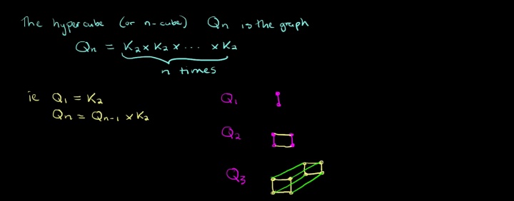
图的笛卡尔积 Cartesian product 是一类重要的图的运算。
1 理论基础
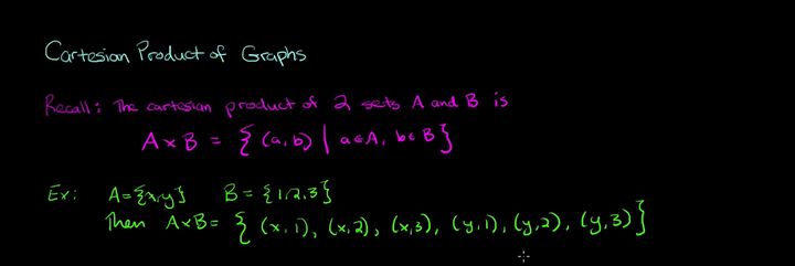
下面是标准的图的笛卡尔积 Cartesian product 定义。
In graph theory , the Cartesian product
-
and
is adjacent to
in
or -
and
is adjacent to
in
.

对于新图的顶点集合怎么得到并不难,不过是做一个简单的顶点集合的笛卡尔积,
首先假设
关键在于新图的边的构造方式的理解。我们单纯看构造边的两个条件,这两个条件地位相等。我们将上述
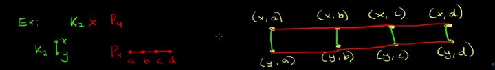
例子1
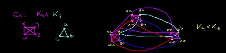
例子2
例子3
有关Cartesian product 性质有很多,不同小方向关心的性质也侧重点也不同,基本的有一些:
The Cartesian product of graphs is sometimes called the box product of graphs [Harary 1969].
The operation is associative, as the graphs
The notation G × H has often been used for Cartesian products of graphs, but is now more commonly used for another construction known as thetensor product of graphs. The square symbol is an intuitive and unambiguous notation for the Cartesian product, since it shows visually the four edges resulting from the Cartesian product of two edges.
2 Maple实现
with(GraphTheory):
G := CycleGraph([v__1,v__2,v__3,v__4]);
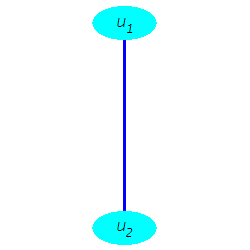
H:=Graph({{u__1,u__2}}):
DrawGraph(C,size=[250,250],stylesheet=[vertexborder=false,vertexpadding=10,
edgecolor = "red",vertexcolor="Orange",
edgethickness=3]);
DrawGraph(H,size=[250,250],stylesheet=[vertexborder=false,vertexpadding=10,
edgecolor = "Blue",vertexcolor="Cyan",
edgethickness=3]);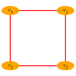
GH:=CartesianProduct(G,H):
plots:-display(
  DrawGraph(GH,style=spring,
            stylesheet=[vertexborder=false,vertexpadding=4,
                        vertexcolor="Orange",edgethickness=3]),
  DrawGraph(GH,style=spring,
            stylesheet=[vertexborder=false,vertexpadding=14,
                        vertexcolor="Cyan",edgethickness=3])
);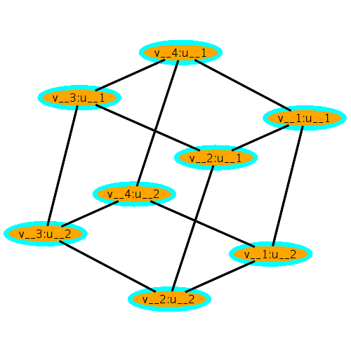
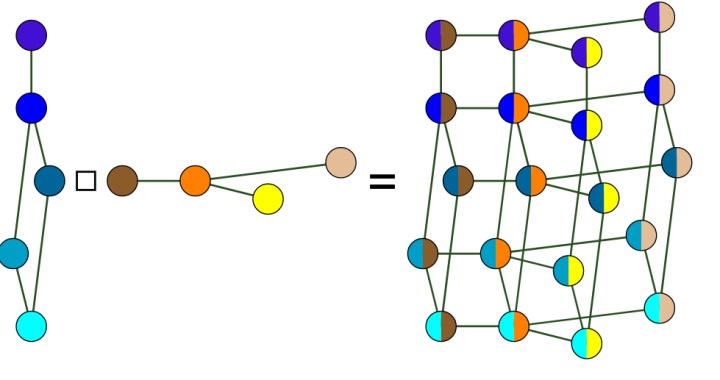
为了便于观察,我们进行了简易修改,这里没有用代码修改了。选中图片右击属性进行适当修改颜色。

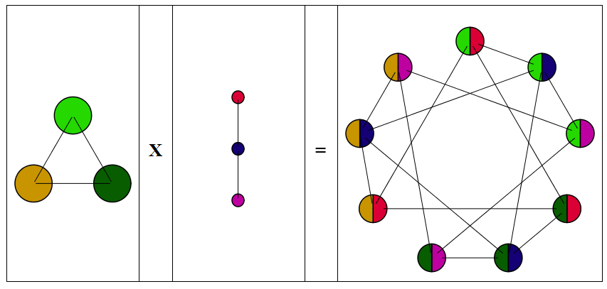
这样图的笛卡尔积演示就出现比较不错的效果。但是达不到题图那样漂亮的效果,我们可以采用下面稍微复杂的代码。
restart:
with(GraphTheory):
with(plots):
randomize():
G1 := Graph({{a, b},{b, c},{c, a}}):
g1 := DrawGraph(G1):

G2 := Graph({{A,B},{B,C}}):
g2 := DrawGraph(G2):

G3 := CartesianProduct(G1, G2):
g3 := DrawGraph(G3):

# Select  the PLOT commands of the edges of each graph
# op(g1) and op(g2) are structured this way:
#   as many POLYGONS commands as vertices
#   as many TEXT commands as vertices
#   as many POLYGONS commands as edges
#   a SCALING command
#   an AXESSTYLE command
#
# Un comment the line below to visualize this
# op(g1);

ne1 := numelems(Edges(G1)):
no1 := nops(g1):
ed1 := op(no1-ne1-1..no1, g1):
PLOT(ed1):

ne2 := numelems(Edges(G2)):
no2 := nops(g2):
ed2 := op(no2-ne2-1..no2, g2):
PLOT(ed2):

ne3 := numelems(Edges(G3)):
no3 := nops(g3):
ed3 := op(no3-ne3-1..no3, g3):
PLOT(ed3):

# Get positions of vertices of each graph

v1 := GetVertexPositions(G1):
v2 := GetVertexPositions(G2):
v3 := GetVertexPositions(G3):

# Get the lengths of the edges of each graph


getlengths := proc(g, no, ne)
  local le, n:
  le := NULL:
  for n from no-ne-1 to no-2 do
    le := le, sqrt(add((`-`(op(op([n, 1], g))))^~2));
  end do:
  return [le]
end proc:
le1 := getlengths(g1, no1, ne1):
le2 := getlengths(g2, no2, ne2):
le3 := getlengths(g3, no3, ne3):

# Find the minimimum lengts  of each graph

mle1 := min(le1):
mle2 := min(le2):
mle3 := min(le3):

# Define the radius of the disk that is going to represent the vertices of each graph

shrink := 4: # to adjust
r1 := mle1 / shrink:
r2 := mle3 / shrink:
r3 := mle3 / shrink:

# Define the colors of these disks for G1 and G2


nv1  := numelems(Vertices(G1)):
col1 := seq([rand()/10^12, rand()/10^12, 0], i=0..nv1-1):
nv2  := numelems(Vertices(G2)):
col2 := seq([rand()/10^12, 0, rand()/10^12], i=0..nv2-1):
nv3  := numelems(Vertices(G3)):

# Vertex disks for G1 and G2

vd1 := display(seq(plottools:-disk(v1[n], r1, color=ColorTools:-Color(col1[n])), n=1..nv1)):
vd2 := display(seq(plottools:-disk(v2[n], r2, color=ColorTools:-Color(col2[n])), n=1..nv2)):

# Vizualize

display(vd1, PLOT(ed1)):
display(vd2, PLOT(ed2)):

# Case of G3: each vertex disk is made of two half disks
# (the cut is choosen to be vertical)

V1 := Vertices(G1):
V2 := Vertices(G2):
V3 := Vertices(G3):

k   := 1:
vd3 := NULL:
for n3 in V3 do
  n1, n2 := StringTools:-Split(op(n3), ":")[]:
  pos1   := ListTools:-Search(parse(n1), V1):
  pos2   := ListTools:-Search(parse(n2), V2):
  vd3    := vd3,
            display(
               plottools:-sector(v3[k], r3, Pi/2..3*Pi/2, color=ColorTools:-Color(col1[pos1])),
               plottools:-sector(v3[k], r3, -Pi/2..Pi/2 , color=ColorTools:-Color(col2[pos2]))
            ):
  k := k+1:
end do:

display(vd3, PLOT(ed3)):

# Compute the rescaling factor of each graph

S1 := sqrt(max(seq(seq(add((v1[i]-~v1[j])^~2), i=j+1..nv1), j=1..nv1-1)));
S1 := sqrt(max(seq(seq(add((v2[i]-~v2[j])^~2), i=j+1..nv2), j=1..nv2-1)));
S1 := sqrt(max(seq(seq(add((v3[i]-~v3[j])^~2), i=j+1..nv3), j=1..nv3-1)));


# Final result

DocumentTools:-Tabulate(
  [
    display(vd1, PLOT(ed1)),
    display(textplot([0, 0, "X"], font=[Tahoma, bold, 20], axes=none)),
    display(vd2, PLOT(ed2)),
    display(textplot([0, 0, "="], font=[Tahoma, bold, 20], axes=none)),
    display(vd3, PLOT(ed3))
  ],
  width=90,
  weights=[4, 1, 4, 1, 8]
):
代码源自于
https://www.mapleprimes.com/questions/230579-Two-Colors-Dye-The-Same-Vertex-Of-Graph?reply=replywww.mapleprimes.com这些演示虽然可能不是研究的重心,真正关心的往往是图运算后一些本质的特征。不过这些基础性的绘图有时候能更好帮助我们理解。
有的图做笛卡尔积之后非常密集,在绘图上几乎看不出连接关系。我们可以采取一些方法。当然这种方案也不是只适用于图笛卡尔积作图。
V := Vertices(GH);
P := [];
flag := 0;
f := proc(K::string) local L; global P; L := Split(K, ":"); P := [op(P), cat("(", L[1], ",", L[2], ")")]; end proc;
if flag = 0 then
    for i to NumberOfVertices(GH) do f(V[i]); end do;
end if;
GH := RelabelVertices(GH, P);
DrawGraph(GH, stylesheet = "legacy")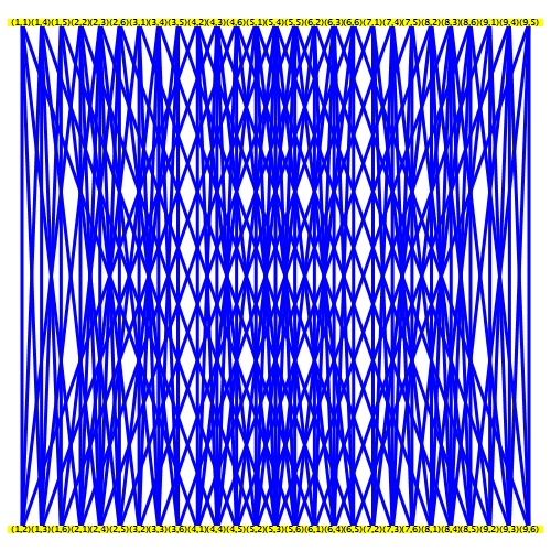
DGR:=DrawGraph(GH, stylesheet = "legacy"):
plots:-display(DGR,scaling=unconstrained,size=[1800,default]);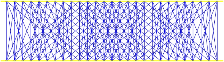
这一做法归功于
https://www.mapleprimes.com/questions/230023-Need-Help-To-Help-DrawGraph-In-Betterwww.mapleprimes.com


 被折叠的 条评论
为什么被折叠?
被折叠的 条评论
为什么被折叠?
 到【灌水乐园】发言


