tf计算矩阵维度_tensorflow计算图与自动求导——tf.GradientTape

最新推荐文章于 2023-06-23 09:41:47 发布

以墨健康道

最新推荐文章于 2023-06-23 09:41:47 发布

阅读量930

点赞数 1

文章标签： tf计算矩阵维度

本文链接：https://blog.csdn.net/weixin_35758901/article/details/112317469

版权

文章共分为4部分

基于计算图的求导
GradientTape 关键方法解析
【注意！】GradientTape 不记录 assign 类操作
高级玩法

1 基于计算图的求导

GradientTape 可以理解为“梯度流记录磁带”：

在记录阶段：记录被 GradientTape 包裹的运算过程中，依赖于 source node （被 watch “监视”的变量）的关系图（计算图）；
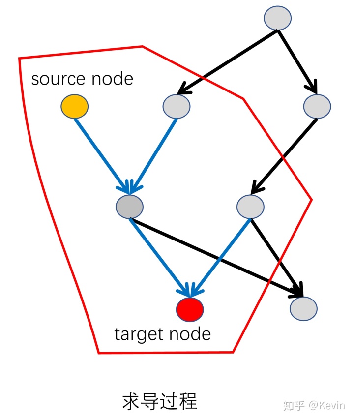
在求导阶段：通过搜索 source node 到 target node 的路径，进而计算出偏微分
。

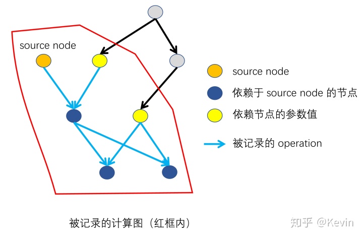
source node 在记录运算过程之前进行指定：

自动“监控”所有可训练变量：GradientTape 默认（watch_accessed_variables=True）将所有可训练变量（created by tf.Variable, where trainable=True）视为需要“监控”的 source node 。
对于不可训练的变量（比如tf.constant）可以使用tape.watch()对其进行“监控”。
此外，还可以设定watch_accessed_variables=False，然后使用tf.watch()精确控制需要“监控”哪些变量。

target node 在求导阶段再指定。

1.1 求导的基本步骤

一阶导

x = tf.constant(3.0)with tf.GradientTape() as g:  # （1）创建一个GradientTape对象
    g.watch(x)  # （2）监视watch要求导的变量
    y = x * x
dy_dx = g.gradient(y, x) # （3）对函数进行求导

二阶导

with tf.GradientTape() as g:
    g.watch(x)
    with tf.GradientTape() as gg:
        gg.watch(x)
        y = x * x
    dy_dx = gg.gradient(y, x)     # 求一阶导数
d2y_dx2 = g.gradient(dy_dx, x)    # 求二阶导数

多阶导数同理

1.2 对同一计算图进行多次求导

GradientTape 默认（persistent = False）在进行一次求导后就销毁计算图，从而节约内存。如果要在同一个计算图下进行多次求导，就要设定 persistent = True 。但是注意要手动释放资源del tape。

x = tf.constant(3.0)
with tf.GradientTape(persistent=True) as g:
  g.watch(x)
  y = x * x
  z = y * y
dz_dx = g.gradient(z, x)  # 108.0 (4*x^3 at x = 3)
dy_dx = g.gradient(y, x)  # 6.0
del g  # Drop the reference to the tape

2 GradientTape 关键方法解析

GradientTape的类结构：

class GradientTape(object):

    def __init__(self, persistent=False, watch_accessed_variables=True):
        """构建函数"""

    def __enter__(self):
        """用于支持with上下文管理器，进入记录的计算图"""

    def __exit__(self, typ, value, traceback):
        """用于支持with上下文管理器，离开计算图"""

    def watch(self, tensor):
        """设定需要“监控”的变量"""

    def stop_recording(self):
        """一个类似with的上下文管理器，tape将不会记录其中的运算操作"""

    def reset(self):
        """清除已有的计算图"""

    def watched_variables(self):
        """返回被“监控”的变量"""

    def gradient(self, target, sources, output_gradients=None,
               unconnected_gradients=UnconnectedGradients.NONE):
        """计算梯度，返回的梯度与 sources 同结构"""

    def jacobian(self, target, sources, unconnected_gradients=UnconnectedGradients.NONE,
               parallel_iterations=None, experimental_use_pfor=True):
        """计算jacobian矩阵"""

    def batch_jacobian(target, source, unconnected_gradients=tf.UnconnectedGradients.NONE,                          parallel_iterations=None, experimental_use_pfor=True):
        """批量计算jacobian"""

init

__init__( persistent=False, watch_accessed_variables=True)
    """构建函数"""

Args:

persistent:

False（默认） : 求导一次后就会自动销毁计算图，不能再求导第二次，这主要是出于节省内存的考虑。

True : 计算图将不会被自动销毁，可以进行多次求导

watch_accessed_variables:

True（默认） : 自动“监控”计算过程中出现的所有可训练变量

False : 需要使用tape.watch()来人为指定需要“监控”的变量

gradient

gradient( target, sources, output_gradients=None,    unconnected_gradients=tf.UnconnectedGradients.NONE)
"""计算梯度，返回的梯度与 sources 同结构"""

Args:

target: Tensor (or list of tensors) 求导的因变量 target node 。
sources: Tensor (or list of tensors) 求导的自变量 sources node 。
unconnected_gradients: 无法求导时，返回的值，有两个可选值["none", "zero"]，默认"none"。例如，当 target node 与 sources node 之间在计算图上没有办法联通时，将会返回None。个人认为，设置为"zero"更合适。

x=tf.Variable(initial_value=[1.0,2.0,3.0])

with tf.GradientTape(persistent=True) as g:
    g.watch(x)
    z=tf.pow(y,2)  # z与x根本就没有关系，即在graph上面没有连接

dz_dx = g.gradient(z, [x,y],unconnected_gradients="none")  # 默认就是none
print(dz_dx)
'''
返回值为：None

由上面可以看出，由于z与x之间并没有连通，所以返回的是None
'''

output_gradients: 对求得的梯度乘以一系列权重，默认为None，不进行操作。其详细用法见下：

x=tf.Variable(initial_value=[1.0,2.0,3.0])

with tf.GradientTape(persistent=True) as g:
    g.watch(x)
    z=tf.pow(x,2)

output_gradients=tf.Variable([-0.2,0.6,0.2])
dz_dx = g.gradient(z, x,output_gradients=output_gradients)   #给每一个元素施加不同的权重
print(dz_dx)
'''运行结果为：
<tf.Tensor: id=64, shape=(3,), dtype=float32, numpy=array([-0.4, 2.4, 1.2], 
  dtype=float32)>

本来的结果是dz_dx=[2,4,6], 分别乘以权重[0.2,0.6,0.2]之后，得到[-0.4,2.4,1.2]
'''

jacobian

jacobian(    target,    sources,    unconnected_gradients=tf.UnconnectedGradients.NONE,    parallel_iterations=None,    experimental_use_pfor=True)
"""计算jacobian矩阵"""

Args:

target：A tensor (or list of tensor) with shape
.
sources: A tensor (or list of tensor) with shape
.
unconnected_gradients: 类似tape.gradient()中的介绍。
parallel_iterations: jacobian的求解中，实际上是含有 while_loop 循环的，而该参数则是允许并行执行的循环个数。该参数将影响内存占用。
experimental_use_pfor:
True（默认） : 使用向量化的方法（pfor）计算 jacobian（vectorizes the jacobian computation）
False : 使用 while_loop 方法计算。
一般来说，向量化能加速计算，但向量化占用的内存远高于 while_loop 。

Returns:

A tensor (or list of tensor) with shape

。

【重点】实际上就是先将 sources x 和 target y “打平”成

和

，求取其 jacobian 矩阵后

，再 reshape 成

的形式。

with tf.GradientTape() as g:
    x = tf.constant(np.random.rand(100, 10, 3))
    W = tf.constant(np.random.rand(100, 3, 5))
    g.watch(x)
    y = x @ W
jacobian = g.jacobian(y, x)

print(jacobian.shape)  # (100, 10, 5, 100, 10, 3)

batch_jacobian

batch_jacobian( target, source, unconnected_gradients=tf.UnconnectedGradients.NONE, parallel_iterations=None, experimental_use_pfor=True)
"""批量计算jacobian"""

批量计算jacobian，相当于：tf.stack([self.jacobian(y[i], x[i]) for i in range(x.shape[0])])。

问题：参考上面jacobian中的例子，直接使用tape.jacobian()也能够计算含有 batch 维度的数据。那么使用tape.batch_jacobian()有什么优势呢？

由于tape.jacobian()会计算所有输入关于输出的 jacobian，而对于含有 batch 维度的数据，显然不同 example 之间是无关的，计算这些无关连接将会产生大量的零矩阵，同时占用大量内存。

Args:

target：A tensor (or list of tensor) with shape
.
sources: A tensor (or list of tensor) with shape
.
unconnected_gradients: 类似tape.gradient()中的介绍。
parallel_iterations、experimental_use_pfor: 类似tape.jacobian()中的介绍。

Returns:

A tensor (or list of tensor) with shape

。

with tf.GradientTape() as g:
    x = tf.constant(np.random.rand(100,10, 3))
    W = tf.constant(np.random.rand(100,3, 5))
    g.watch(x)
    y = x @ W
jacobian = g.batch_jacobian(y, x)

print(jacobian.shape)  # (4, 10, 5, 10, 3)

reset

reset()
"""清除已有的计算图"""

下面两个代码块是等价的：

with tf.GradientTape() as t:  
    loss = loss_fn()
with tf.GradientTape() as t: 
    loss += other_loss_fn()
t.gradient(loss, ...)  # Only differentiates other_loss_fn, not loss_fn

# The following is equivalent to the above

with tf.GradientTape() as t:  
    loss = loss_fn() 
    t.reset()  
    loss += other_loss_fn()t.gradient(loss, ...)  # Only differentiates other_loss_fn, not loss_fn

问题：既然有上面的等价形式，那么tape.reset()是不是就是多余的呢？

当然不是啦，利用reset可以在同一个tape里面进行不同计算图的切换：

loss = 0.0
with tf.GradientTape() as t: 
    loss += encoder_loss_fn()  
    if use_decoder == True:    
        t.reset()
        loss += decoder_loss_fn()

虽然用等价形式也可以做到，但是用reset显然更漂亮，漂亮就是最大的用处。

stop_recording

stop_recording()
"""一个类似with的上下文管理器，tape将不会记录其中的运算操作"""

利用该函数，可以选择不记录某些运算操作，从而节省内存。还可以实现计算图的中断（见 3.1 截断的计算图）。

with tf.GradientTape(persistent=True) as t:    
    loss = compute_loss(model)    
    with t.stop_recording():      # The gradient computation below is not traced, saving memory.
        grads = t.gradient(loss, model.variables)

watch

watch(tensor)
"""设定需要“监控”的变量"""

Args:

tensor: 一个tensor，或者tensor的列表

watched_variables

watched_variables()
"""返回被“监控”的变量"""

3 【注意！】GradientTape 不记录 assign 类操作

在 tf2.0 中，删除了tf.下的所有 assign 类函数，包括tf.assign()、tf.assign_add()、tf.assign_sub()等。但是仍保留了tf.Variable.下的 assign 类函数。

3.1 assign 与 `=` 的区别

如果不深入了解 assign 类函数函数的运行方式，就很容易陷入一个常见误区，亦即误以为 assign 操作与=操作是等价的：

''' assign 操作 '''
a.assign(b)
a.assign_add(b)
a.assign_sub(b)
''' = 操作 '''
a = b
a = a + b
a = a - b

上面两种操作虽然计算结果相等，但在计算图上的作用是完全不同的。现在以下面的两个变量a、b和计算图节点'a:0'、'b:0'为例进行分析：

a=tf.Variable([1,2,3],name='a')
# a:  <tf.Variable 'a:0' shape=(3,) dtype=int32, numpy=array([1, 2, 3])>
b=tf.Variable([4,5,6],name='b')
# b:  <tf.Variable 'b:0' shape=(3,) dtype=int32, numpy=array([4, 5, 6])>

a.assign(b)：a仍然指向'a:0'节点，计算图上依然只有'a:0'和'b:0'两个节点。虽然'a:0'的值变为'b:0'的值，但是两个节点之间没有建立依赖关系。（对于其他 assign 类操作同理）

a.assign(b)
# a:  <tf.Variable 'a:0' shape=(3,) dtype=int32, numpy=array([4, 5, 6])>
'''
a --> 'a:0' [4, 5, 6]
      'b:0' [4, 5, 6]
'''

a = b：计算图保持不变，没有建立任何依赖关系，a改为指向'b:0'节点。

python a = b # a: <tf.Variable 'b:0' shape=(3,) dtype=int32, numpy=array([4, 5, 6])> ''' 'a:0' [1, 2, 3] a --> 'b:0' [4, 5, 6] '''

a = a + b：计算图新增一个依赖于'a:0'和'b:0'的节点'id=2185'，a改为指向新节点'id=2185'。（对于a = a - b同理）

a = b
# a:  <tf.Variable 'b:0' shape=(3,) dtype=int32, numpy=array([4, 5, 6])>
'''
      'a:0' [1, 2, 3]
a --> 'b:0' [4, 5, 6]
'''

总的来说：

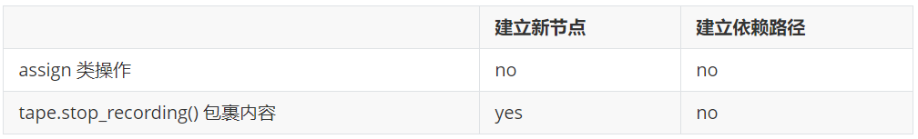
assign 操作：仅改变计算图中某个节点的值，不改变计算图结构（不新建节点，不新建依赖路径）。
运算式 a = func(b,c...) ：在计算图中创建一个新节点来记录计算结果，同时建立b,c...指向的节点到新节点的依赖关系。
赋值a = b：计算图不变，a、b同时指向原来b指向的节点。
注：如果要达到运算式a = identity(b)的效果（亦即新建一个节点，使其依赖于b指向节点，并且两节点同值），可以使用a = tf.identity(b)。

3.2 assign 会造成梯度断流

由上面分析可知， assign 操作不建立节点间的依赖关系，这就导致 assign 操作无法传递梯度。

with tf.GradientTape() as tape:
    tape.watch([a])
    a.assign_add(b)

db_da = tape.gradient(b, a)
print(db_da)
'''
None  
'''

利用这种特性，我们可以设计截断的计算图（参照 4.1 截断的计算图）。

3.3 assign 与 tape.stop_recording() 的区别

assign :

with tf.GradientTape(persistent=True) as tape:
    tape.watch([a])
    a.assign_add(b)

db_da = tape.gradient(b, a)
del tape
print(db_da)
print(a, b)
'''
None
<tf.Variable 'a:0' shape=(3,) dtype=int32, numpy=array([5, 7, 9])>
<tf.Variable 'b:0' shape=(3,) dtype=int32, numpy=array([4, 5, 6])>
'''

tape.stop_recording() :

with tf.GradientTape(persistent=True) as tape:
    tape.watch([a])
    with tape.stop_recording():
        a = a + b

db_da = tape.gradient(b, a)
del tape
print(db_da)
print(a, b)
'''
None
tf.Tensor([5 7 9], shape=(3,), dtype=int32)  # 新建节点
<tf.Variable 'b:0' shape=(3,) dtype=int32, numpy=array([4, 5, 6])>
'''

4 高级玩法

4.1 截断的计算图

以下面的运算式为例：

则z对x的偏导为

，如果仅仅想求取z对x的立即导数

，则需要建立了一个截断的计算图，解除y对x的依赖。

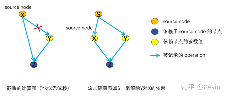
如上图所示，共有两种方式实现：

不记录依赖路径上

'''使用 tape.stop_recording()'''
x = tf.Variable(4.0)
with tf.GradientTape() as g:
    g.watch(x)
    with g.stop_recording():
        y = x * x
    z = x + y
grads_1 = g.gradient(z, x)
'''grads_1 = 1.0'''

'''使用 assign 操作'''
x = tf.Variable(4.0)
y = tf.Variable(0.0)
with tf.GradientTape() as g:
    g.watch(x)
    y.assign(x * x)
    z = x + y
grads_1 = g.gradient(z, x)
'''grads_1 = 1.0'''

添加隐藏节点来解除依赖关系

s = tf.Variable(4.0)
with tf.GradientTape() as g:
    g.watch(s)
    x = tf.identity(s)
    y = s * s
    z = x + y
grads_2 = g.gradient(z, x)
'''grads_2 = 1.0'''

【注意！】对于方式（2），赋值操作要使用x = tf.identity(s)而不能用x = s，因为后者不新建节点，只是让变量x指向s所指向的节点。

以墨健康道

关注

1
点赞
踩
3

收藏

觉得还不错? 一键收藏
0
评论
tf计算矩阵维度_tensorflow计算图与自动求导——tf.GradientTape

文章共分为4部分基于计算图的求导GradientTape 关键方法解析【注意！】GradientTape 不记录 assign 类操作高级玩法1 基于计算图的求导GradientTape 可以理解为“梯度流记录磁带”：在记录阶段：记录被 GradientTape 包裹的运算过程中，依赖于 source node （被 watch “监视”的变量）的关系图（计算图）；在求导阶段：通过搜索 sour...
复制链接

扫一扫