莫兰指数stata命令_基于Stata的ESDA（探索性空间数据分析）代码解析与实操验证...

一、引言

探索性空间数据分析(Exploratory Spatial Data Analysis，ESDA)是空间计量经济学的重要技术。

网上调研发现，鲜有基于Herrera Gomez(2016)的方法，使用中国本土数据，比较全面地实现ESDA的文章。本文可能是中国第一篇基于中国本土数据，实现Herrera Gomez(2016)技术，并对其进行深度解读的文章。

本文由五大部分组成：第一部分为引言。第二部分为空间权重矩阵的生成。第三部分为Univariate Spatial Tests，包括：使用不同软件和命令计算单变量全域莫兰指数，绘制单变量莫兰散点图；热点分析(Hot Spot Analysis)的实现。第四部分为Choropleth Map，包括：绘制Quantile Map、Equal Intervals Map、Box Map、Deviation Map及Combine Map。

二、生成空间权重矩阵

ASEF已经推送过，很多关于如何生成各种空间权重矩阵的文章或视频。感兴趣的朋友，可以在ASEF公众号的“文章分类”中进行查找。在这里，不再演示如何生成空间权重矩阵。

需要说明的是：本文所有演示采用的矩阵均为距离倒数空间权重矩阵(inverse of the squared distance weight matrix)。

三、Univariate Spatial Tests

(一)计算Moran's I

1.计算全域Moran's I

. use winv.dta,clear

. spatwmat using winv.dta,name(winv)standardize

. use ti&ts_34variables.dta,clear

.spatgsati_2002 ti_2003 ti_2004 ti_2005 ti_2006 ti_2007 ti_2008 ti_2009 ti_2010 ti_2011 ti_2012ti_2013 ti_2014 ti_2015 ti_2016 ti_2017 ti_2018 ,weights(winv) moran，见图1

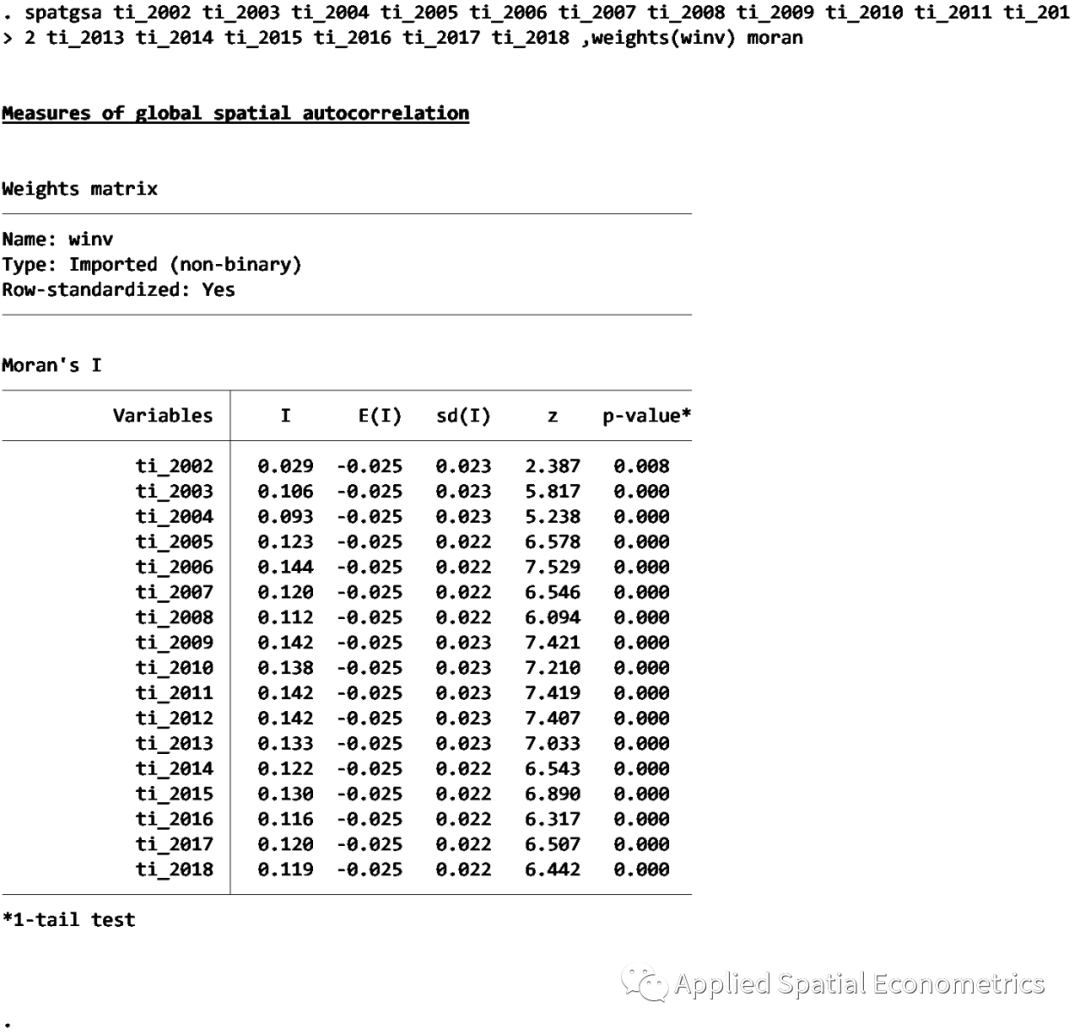
图1

2.计算局域Moran's I

. use winv.dta

. spatwmat using winv.dta,name(winv)standardize

. use ti&ts_34variables,clear

. spatlsa ti_2018, w(winv) moran twotail，见图2

图2

(二)画Moran’s I散点图

1.GeoDa绘制的莫兰散点图

基于GeoDa求全域莫兰指数，绘制莫兰散点图，操作非常简单。详见ASEF前期推文。GeoDa求莫兰指数的一个缺点是：一次只能求一个年份的Global Moran's I。在此方面，Stata具有优势，它一次可以求出所有年份的Global Moran's I。

2.Stata绘制的莫兰散点图

(1)spatlsa命令绘制的莫兰散点图

. use winv.dta,clear

. spatwmat using winv.dta,name(winv)standardize

. use ti&ts_34variables,clear

. spatlsa ti_2018,weights(winv) morangraph(moran) symbol(id)id(cm)，见图3与图4

. spatlsa ti_2018,weights(winv) morangraph(moran) symbol(id)id(cm) twotail

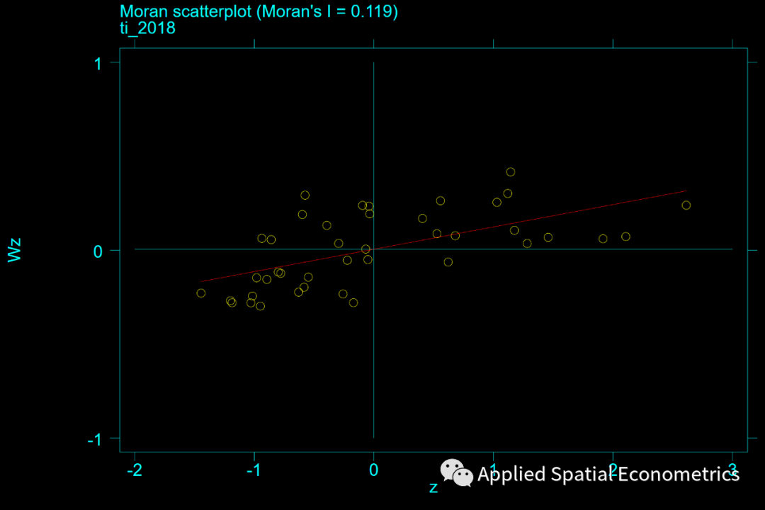
图3

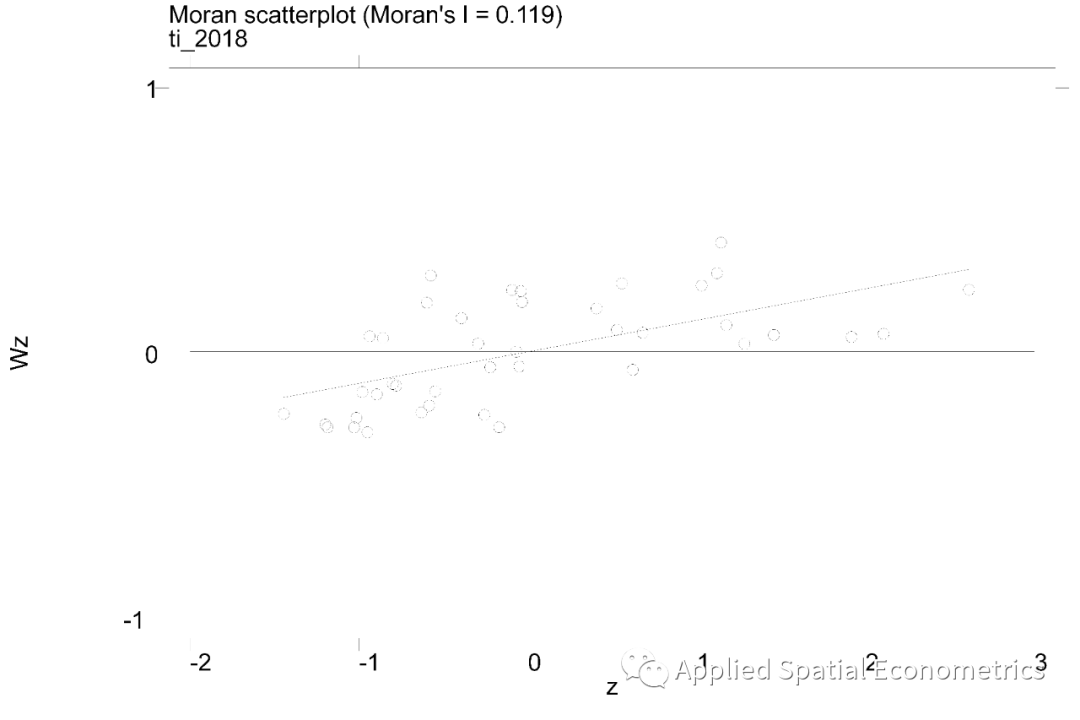
图4

(2)splagvar命令绘制的sophisticated 莫兰散点图

. use winv.dta,clear

. spatwmat using winv.dta,name(winv)standardize

. use ti&ts_34variables,clear

. splagvar ti_2018, wname(winv) wfrom(Stata) ind(ti_2018)order(1) plot(ti_2018) moran(ti_2018)，见图5

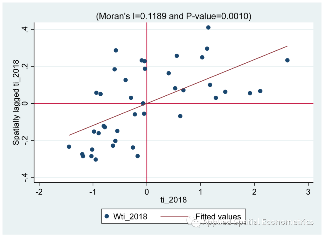
图5  基于splagvar命令绘制的sophisticated 莫兰散点图

注：本文的一个重要贡献是，在中国较早的公开了splagvar命令绘制的sophisticated 莫兰散点图的命令和代码。

*绘制Local Moran’s I图

. genmsp ti_2018, w(W)

. graph twoway (scatter Wstd_ti_2018 std_ti_2018 if pval_ti_2018>=0.05,msymbol(i)  mlabel (id) mlabsize(*0.6)mlabpos(c)) (scatter Wstd_ti_2018 std_ti_2018 if pval_ti_2018<0.05,msymbol(i) mlabel (id) mlabsize(*0.6) mlabpos(c) mlabcol(red)) (lfit Wstd_ti_2018std_ti_2018), yline(0, lpattern(--)) xline(0, lpattern(--)) xlabel(-1.3(1)2.6,labsize(*0.8)) xtitle("{it:z}") ylabel(-5.0(2.5)10.0, angle(0)labsize(*0.8)) ytitle("{it:Wz}") legend(off) scheme(s1color)title("Local Moran I of ti_2018")，见图6

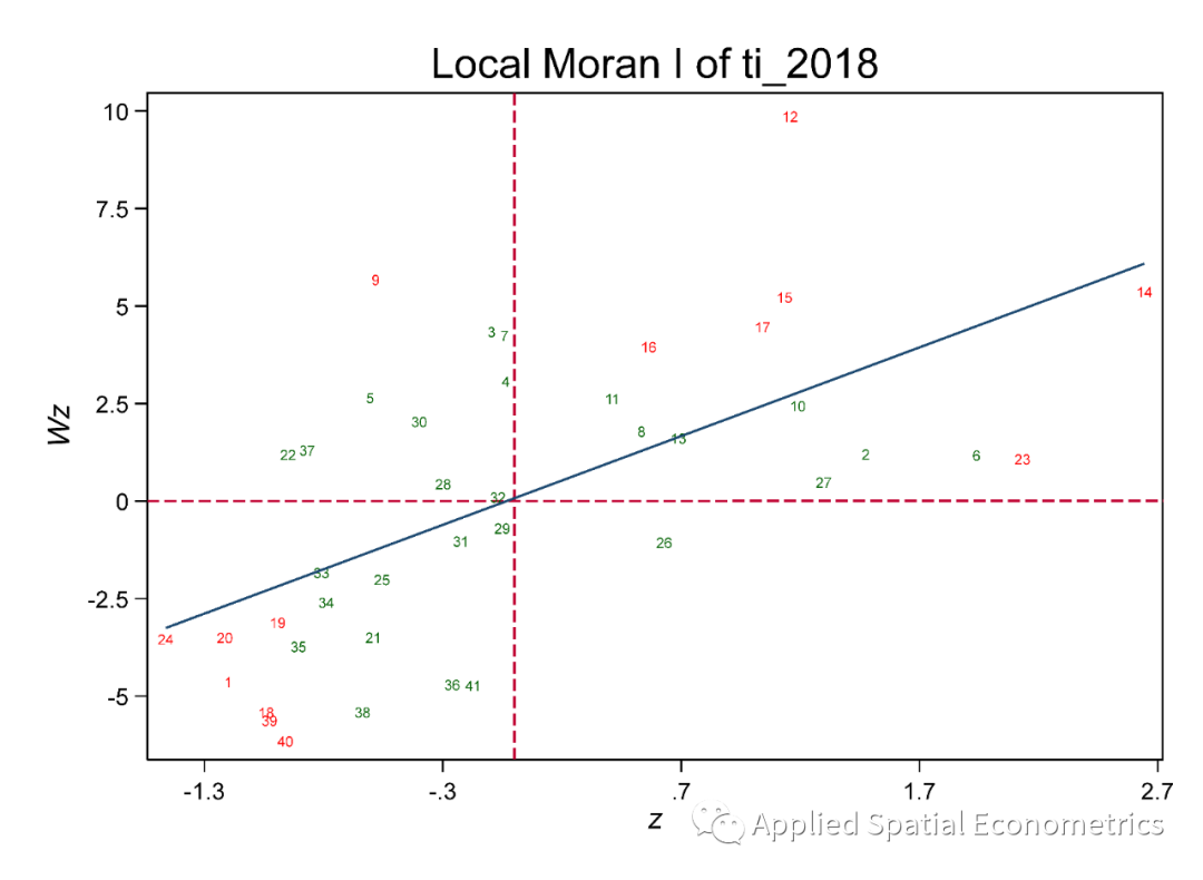
图6 

四、Choropleth Map

(一)Quantile map

. shp2dta using ti&ts_34variables,database(data_shp) coordinates(coord) genid(id) genc(c)

. use data_shp,clear

. spmap ti_2018 using coord, id(id) clmethod(q) title (`"  {fontface "stSerif":2018} {fontface"宋体":年长江三角洲地区} {fontface "stSerif":TI} {fontface "宋体":空间分位图}"')legend(size(small) position(8)) fcolor(BuRd) note("Source: China Statistical Yearbook")

同时使用Times New Roman和宋体。position(8)，其中，()里的数据表示方位。见图7。

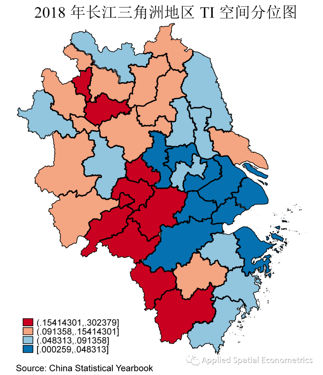
图7

(二)Equal Intervals Map

. spmap ti_2018using coord, id(id) clmethod(e)title (`"  {fontface "stSerif":2018} {fontface"宋体":年长江三角洲地区} {fontface "stSerif":TI Equal Intervals Map } "') legend(size(small) position(8)) fcolor(BuRd) note("Source: China Statistical Yearbook")，见图8

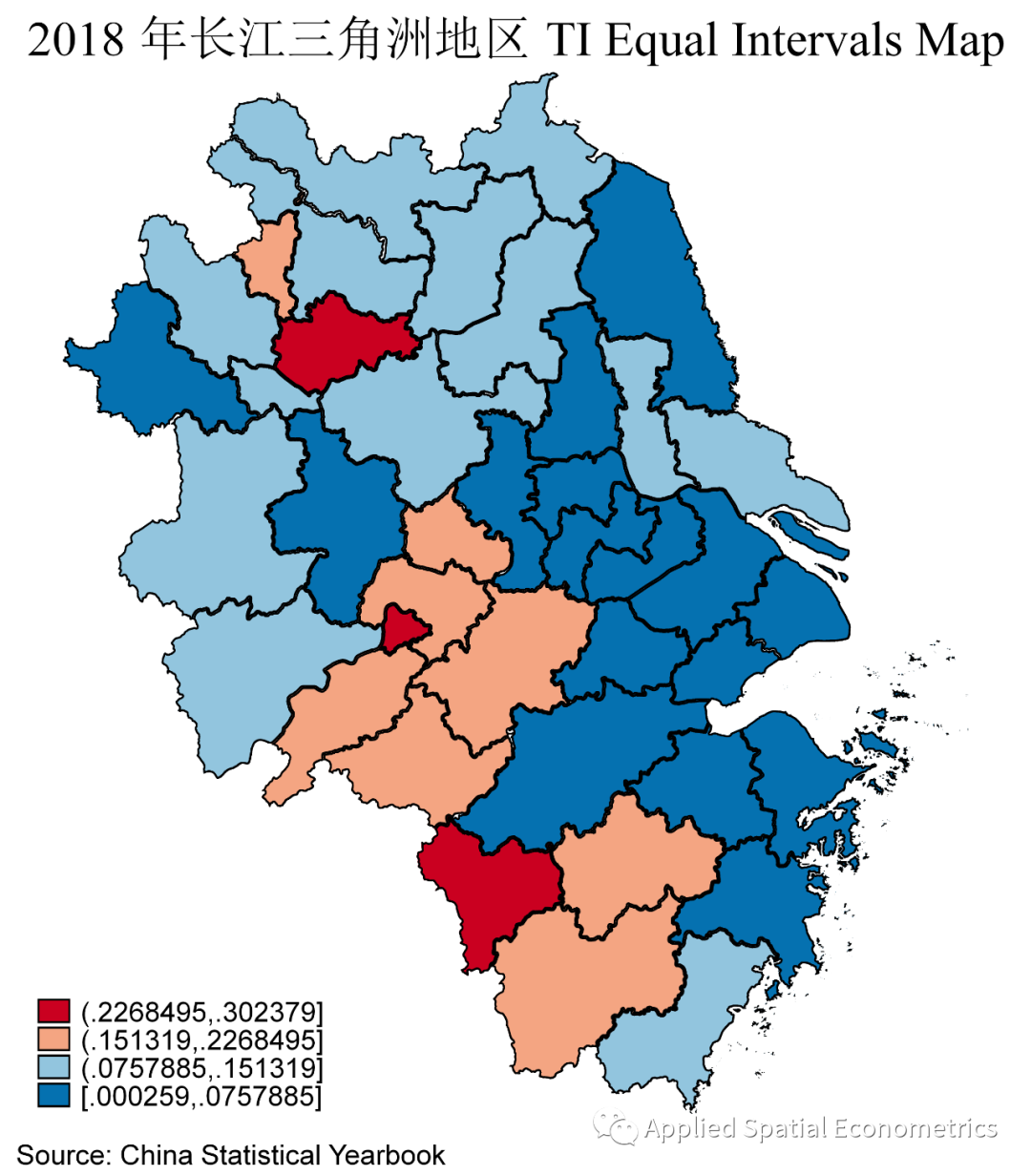
图8

(三)Box Map

. use data_shp,clear

. spmap ti_2018using coord, id(id) clmethod(boxplot)  title (`"  {fontface"stSerif":2018} {fontface "宋体":年长江三角洲地区} {fontface"stSerif":TI Box Map}"') legend(size(small) position(8)) fcolor(Heat) note( "Source: China Statistical Yearbook")，见图9

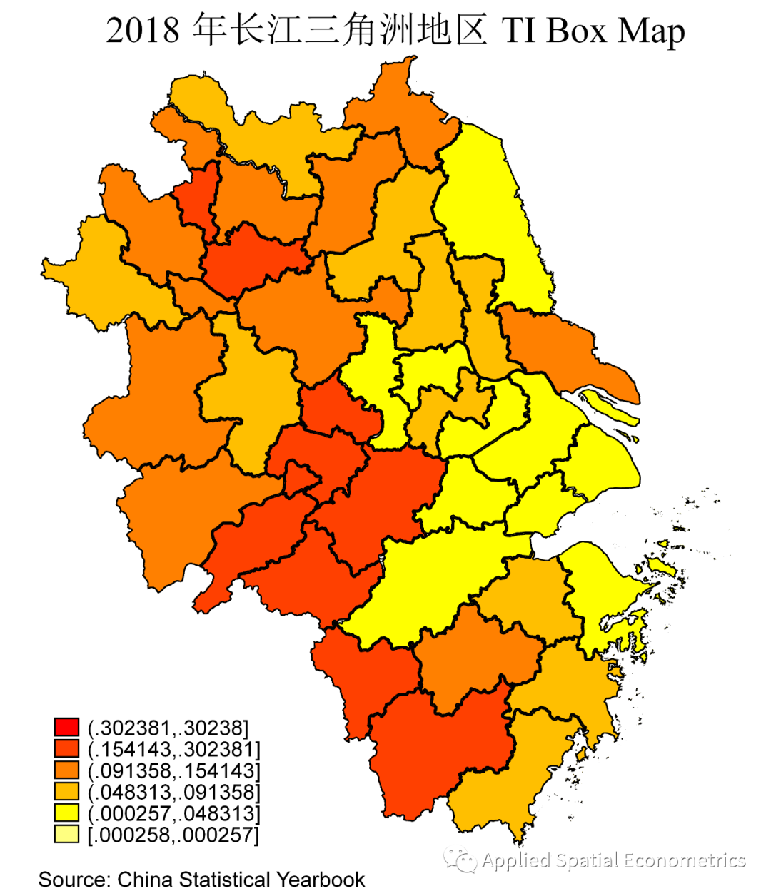
图9

. graph hbox ti_2018, asyvars ytitle("ti_2018")，见图10

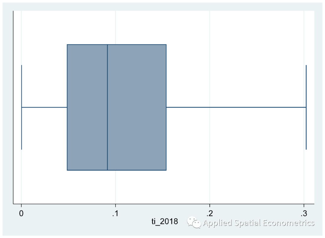
图10

(四)Deviation Map

. spmap ti_2018 using coord, id(id) clmethod(s) title(`"  {fontface"stSerif":2018} {fontface "宋体":年长江三角洲地区} {fontface "stSerif":TI Deviation Map}"')legend(size(small) position(8)) fcolor(BuRd) note( "Source: ChinaStatistical Yearbook")，见图11

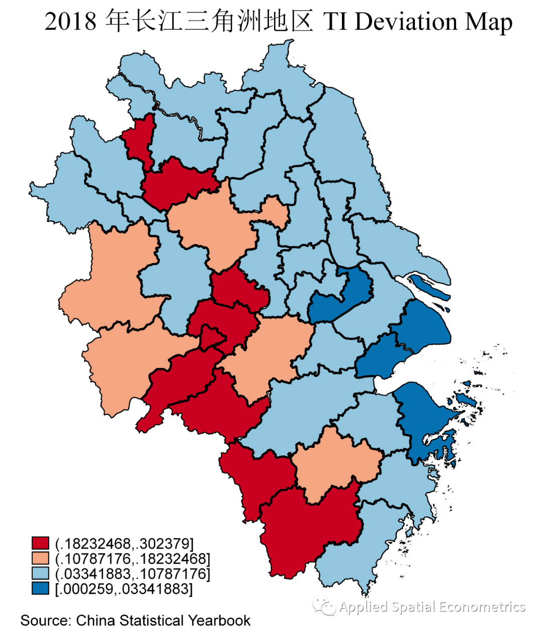
图11

(五)Combine Map

. spmap ti_2018using coord, id(id) fcolor(RdYlBu) cln(5) point(data(data_shp) xcoord(x_c)ycoord(y_c) deviation( ti_2018) sh(T) fcolor(dknavy) size(*0.3)) legend(size(small)position(8)) legt(`"  {fontface "stSerif":2018} {fontface"宋体":年长江三角洲地区} {fontface "stSerif":TI} "') note(" " "Solid triangles indicate values over themean of TI."  "Source: China Statistical Yearbook")，见图12

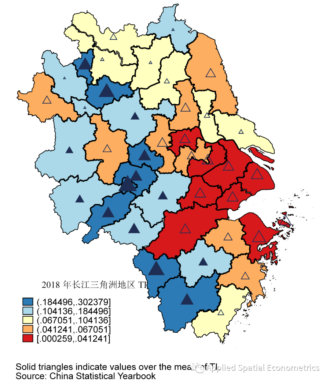
图12

. spmap ti_2018using coord, id(id) fcolor(RdYlBu) cln(5) diagram(var(ti_2018) xcoord(x_c)ycoord(y_c) fcolor(gs2) size(1.7)) legend(size(small) position(8)) legstyle(3) legt(2018年长江三角洲地区TI) note("Boxes indicate values of TI."  "Source: China Statistical Yearbook")，见图13

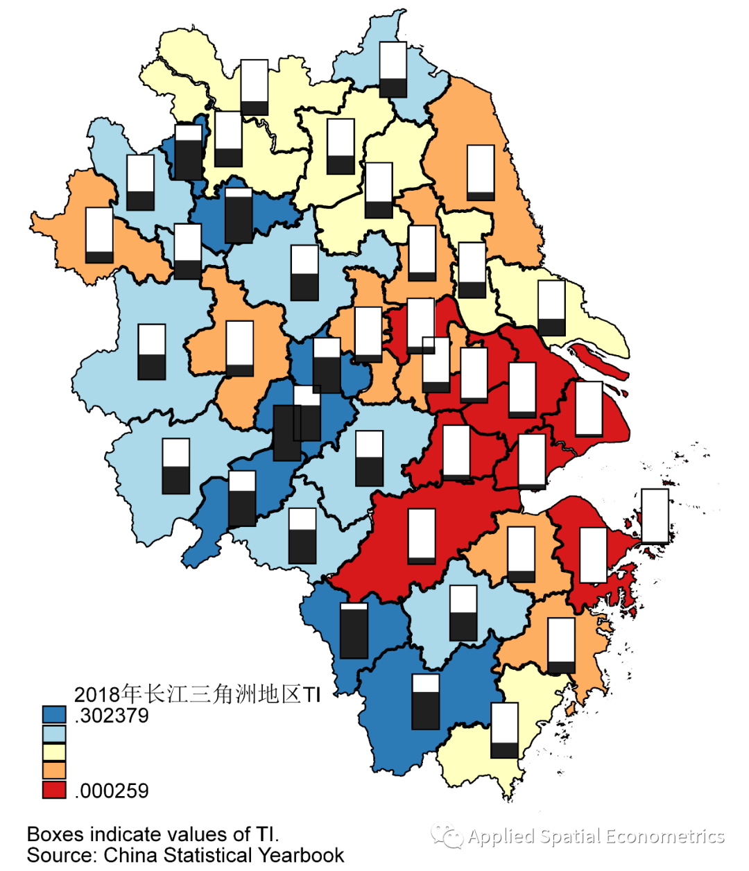
图13

五、结束语

为满足不同空间计量爱好者的需求，后续，ASEF会推送此文的视频版。感谢您一直以来对ASEF的关心、鼓励及支持！

为了进一步方便广大空间计量爱好者进行学习、交流及合作，该微信公众号申请了一个ASEF微信交流群。该群直属于ASEF微信公众号。感兴趣的朋友可以添加孙攀博士的微信(微信号：teenchee)，让他邀请您进入ASEF微信交流群。

孙攀，公众号：Applied Spatial EconometricsASEF：使命、定位及目标

参考文献：

[1]  Anselin,L. and Bera, A.K. (1998) Spatial Dependence in Linear Regression Models with anIntroduction to Spatial Econometrics. Statistics: Textbooks and Monographs,155, 237-289.

[2]  Brueckner,J. K. (2003). Strategic Interaction Among Governments: An Overview of EmpiricalStudies. International Regional Science Review, 26(2), 175–188.

[3]  Ertur,Cem & Koch, Wilfried. (2007). Growth, Technological Interdependence andSpatial Externalities: Theory and Evidence. Journal of Applied Econometrics.22. 1033-1062.

[4]  LeGallo, Julie & Ertur, Cem. (2003). Exploratory Spatial Data Analysis of theDistribution of Regional Per Capita GDP in Europe, 1980–1995. Journal ofEconomics. 82. 175-201.

[5]  Fingleton,Bernard. (2006). A cross-sectional analysis of residential property prices: Theeffects of income, commuting, schooling, the housing stock and spatial interactionin the English regions. Papers in Regional Science. 85. 339-361.

[6]  Anselin,L. (1988). Spatial Econometrics: Methods and Models. LeSage, J. and Pace(2009). An introduction to spatial econometrics.

[7]  Elhorst,J. P. (2014). Spatial econometrics: from cross-sectional data to spatial panels.

[8]  Belotti,F. et al (2016). XSMLE: Stata module for spatial panel data models estimation.Statistical Software Components.

[9]  Drukker,D. M. et al. (2011). A command for estimating spatial-autoregressive modelswith spatial-autoregressive disturbances and additional endogenous variables.Econometric Reviews, 32, 686-733.

[10]  Drukker,D. M. et al. (2013). Creating and managing spatial-weighting matrices with thespmat command. Stata Journal, 13(2), 242-286.

[11]  Pisati,M. (2008). SPMAP: Stata module to visualize spatial data. Statistical SoftwareComponents.

[12]  HerreraGomez, Marcos. (2017). Spatial Econometrics Methods using Stata.10.13140/RG.2.2.16430.92489.

Focuses on the Setting and Application of Spatial Econometric Models, and Commits to Promote the Development of Spatial Econometrics in China.