


Exercise 11.1: Plotting a function
这道题比较简单,画出一个函数的图像即可,算出10000个函数节点的值,再用plot画出图像即可。
import numpy as np
import matplotlib.pyplot as plt

x = np.linspace(0,2,10000)
y = np.power(np.sin(x-2),2)
temp1 = np.power(x,2)
temp2 = np.exp(-1 * temp1)
y = y * temp2;
plt.plot(x,y)
#print(y)
#print(x)
#加入坐标轴相关信息
plt.xlabel("My x lable")
plt.ylabel("My y lable")
plt.title("Exercise 11.1: Plotting a function")
plt.show()
Exercise 11.2: Data
这道题要使用计算最小二乘法,并画出估计出的系数矩阵的图像和真实的系数矩阵的图像。
import numpy as np
import matplotlib.pyplot as plt

X = np.random.rand(20,10)
b = np.random.rand(10)
z = np.random.normal(size=20)
y = X.dot(b)+z
#使用最小二乘法求b
n1 = (X.T).dot(X)
n2 = (X.T).dot(y)
b1 = np.linalg.inv(n1).dot(n2)
print(b1)
x = np.linspace(0,9,10)
fig = plt.figure()
a1 = fig.add_subplot(111)
a1.scatter(x,b,c = 'r',marker = 'o')
a1.scatter(x,b1,c = 'b',marker = '>')
a1.set_title('Exercise 11.2')
plt.xlabel('X')
plt.ylabel('Y')
plt.legend('TE')
plt.show()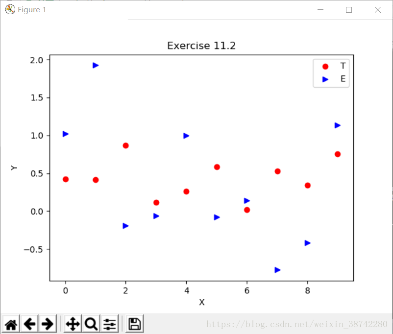
Exercise 11.3: Histogram and density estimation
这道题要画出z的histogram并且使用核密度估计法估计密度并且作图,将开发手册中的gaussian_kde中的实例稍作更改即可实现
import numpy as np
import matplotlib.pyplot as plt
from scipy.stats import gaussian_kde

x = np.random.normal(size = 1000)
y = np.random.normal(size = 1000)
xy = np.vstack([x,y])
z = gaussian_kde(xy)(xy)
f,(ax1,ax2) = plt.subplots(1,2,figsize=(6,3))
ax1.hist(x, bins = 30, normed = True, color = 'b')
ax2.scatter(x,y,c=z,s=100,edgecolor='')
plt.show()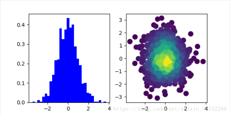


 2959
2959

 被折叠的 条评论
为什么被折叠?
被折叠的 条评论
为什么被折叠?
 到【灌水乐园】发言


