barplot参数 python_Python可视化22|Seaborn.catplot(下)-boxenplot|barplot

本文介绍Seaborn.catplot中的 boxenplot|barplot|countplot图

本文速览

欢迎随缘关注@pythonic生物人

seaborn分栏条形图

seaborn增强箱图图

目录

7、seaborn. boxenplot（增强箱图）
不分类增强箱图boxenplot
分类增强箱图
scale参数
k_depth参数
8、 seaborn. barplot（条形图或柱状图）
分类barplot
分类水平barplot
误差棒属性设置
渐变色调色盘
所有柱子一个颜色
更个性化设置
多重分类barplot
catplot()结合 barplot()和FacetGrid 绘制多子图
9、seaborn. countplot
不分类countplot
分类countplot
catplot()结合countplot和FacetGrid绘制多子图

---

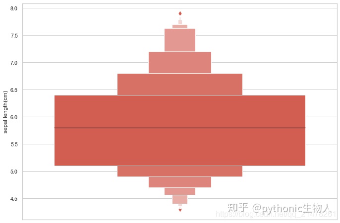
7、seaborn.boxenplot（增强箱图）

该图为boxplot的加强版，提供更多数据的分布信息【箱子更多了】
语法：seaborn.boxenplot(x=None, y=None, hue=None, data=None, order=None, hue_order=None, orient=None, color=None, palette=None, saturation=0.75, width=0.8, dodge=True, k_depth='proportion', linewidth=None, scale='exponential', outlier_prop=None, showfliers=True, ax=None, **kwargs)
介绍一些特异参数

• 不分类增强箱图boxenplot

#sepal length(cm)不分类增强箱图boxenplot
plt.figure(dpi=70)
sns.set(style="whitegrid")
sns.boxenplot(y='sepal length(cm)',data=pd_iris,#传入数据pd_iris第一列
              palette=["#e74c3c", "#34495e", "#2ecc71"],
             )

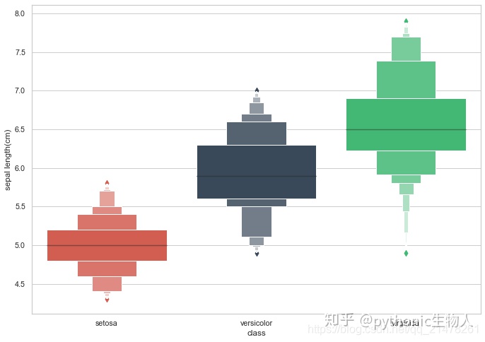
• 分类增强箱图

#按class分类增强箱图
plt.figure(dpi=70)
sns.set(style="whitegrid")
sns.boxenplot(y='sepal length(cm)',x='class',data=pd_iris1,
              palette=["#e74c3c", "#34495e", "#2ecc71"], 
             )

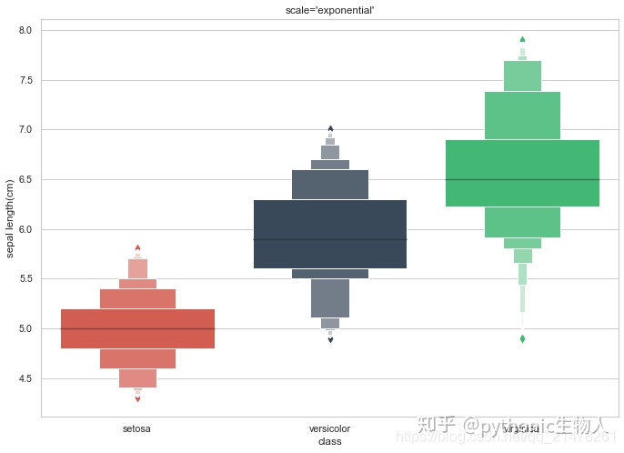
• scale参数

即箱子呈现模式，可选linear( reduces the width by a constant linear factor),
exponential（默认,uses the proportion of data not covered）,
area(proportional to the percentage of data covered，和exponential想反)

#scale参数
for i in list('area,linear,exponential'.split(',')):
    plt.figure(dpi=70)
    sns.set(style="whitegrid")
    sns.boxenplot(y='sepal length(cm)',x='class',data=pd_iris1,
                   palette=["#e74c3c", "#34495e", "#2ecc71"],
                   scale='%s'%i
                  )
    plt.title("scale='%s'"%i)

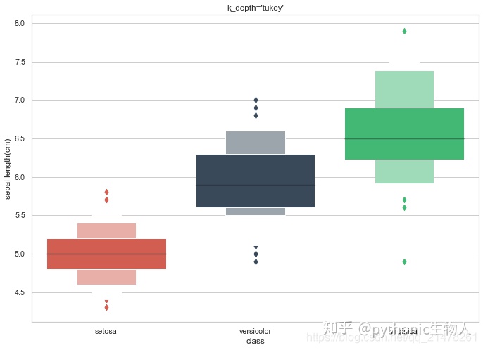
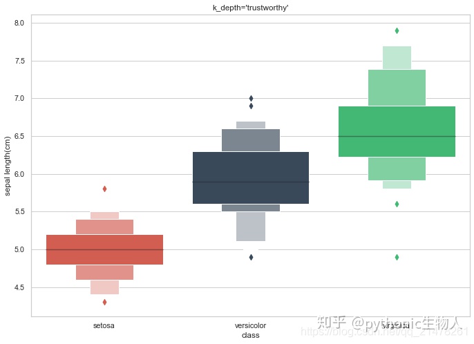
• k_depth参数

#k_depth参数
for i in list('proportion,tukey,trustworthy'.split(',')):
    plt.figure(dpi=70)
    sns.set(style="whitegrid")
    sns.boxenplot(y='sepal length(cm)',x='class',data=pd_iris1,
                   palette=["#e74c3c", "#34495e", "#2ecc71"],
                   k_depth='%s'%i#箱子数量控制，可选proportion（默认）,tukey,trustworthy
                  )
    plt.title("k_depth='%s'"%i)

---

8、 seaborn.barplot（条形图或柱状图）

更基础的更个性化的玩法，参考 ：Python可视化|matplotlib12-垂直|水平|堆积条形图详解语法：seaborn.barplot(x=None, y=None, hue=None, data=None, order=None, hue_order=None, estimator=<function mean at 0x105c7d9e0>, ci=95, n_boot=1000, units=None, seed=None, orient=None, color=None, palette=None, saturation=0.75, errcolor='.26', errwidth=None, capsize=None, dodge=True, ax=None, **kwargs)

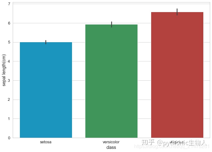
• 分类barplot

#按class分类barplot
plt.figure(figsize=(8,5))
sns.set(style="whitegrid",font_scale=1.2)
sns.barplot(y='sepal length(cm)',x='class',data=pd_iris1,
              palette=["#01a2d9","#31A354","#c72e29"], 
             )

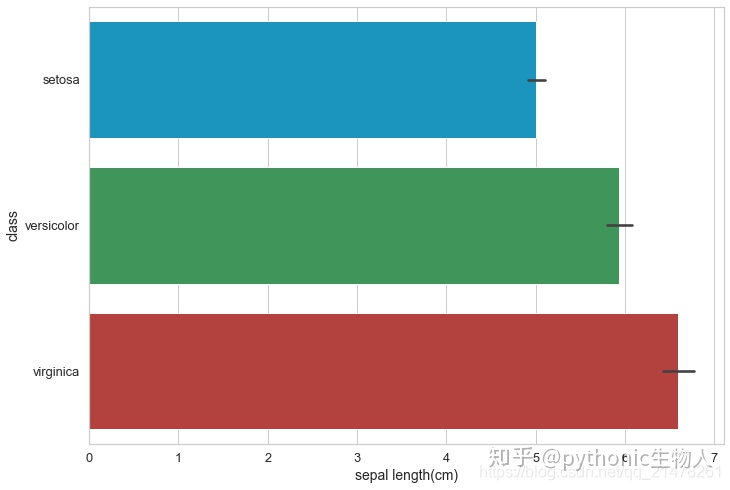
• 分类水平barplot

#按class分类水平barplot
plt.figure(dpi=70)
sns.set(style="whitegrid",font_scale=1.2)
sns.barplot(x='sepal length(cm)',y='class',data=pd_iris1,#将x和y变量换下就可以
              palette=["#01a2d9","#31A354","#c72e29"], 
             )

• 误差棒属性设置

#误差棒属性设置
plt.figure(dpi=70)
sns.set(style="whitegrid",font_scale=1.2)
sns.barplot(y='sepal length(cm)',x='class',data=pd_iris1,
              palette=["#01a2d9","#31A354","#c72e29"],
            ci='sd',#设置误差棒的置信区间，可选'sd',float（默认95，即95%置信区间）
            errcolor='#c72e29',#误差棒颜色
            errwidth=6,#误差棒宽度
            capsize=0.05,#误差棒上下横线长度            
            
             )

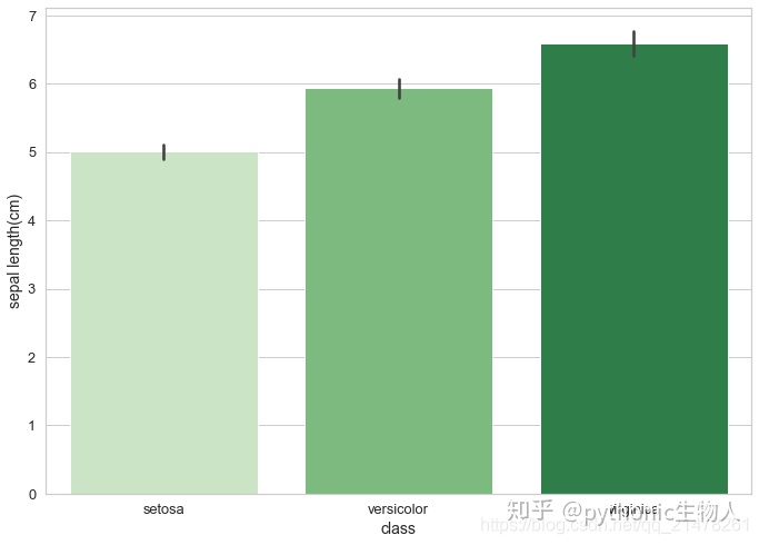
• 渐变色调色盘

#渐变色调色盘
plt.figure(dpi=70)
sns.set(style="whitegrid",font_scale=1.2)
sns.barplot(y='sepal length(cm)',x='class',data=pd_iris1,
              palette='Greens',
             )

• 所有柱子一个颜色

#所有柱子一个颜色
plt.figure(dpi=70)
sns.set(style="whitegrid",font_scale=1.2)
sns.barplot(y='sepal length(cm)',x='class',data=pd_iris1,
            color='#d5695d',#单独颜色
            saturation=.4,#饱和度
             )

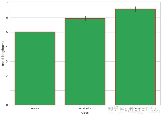
• 更个性化设置

参考matplotlib.axes.Axes.bar()中参数

#更多参数设置matplotlib.axes.Axes.bar()中参数
plt.figure(dpi=70)
sns.set(style="whitegrid",font_scale=1.2)
sns.barplot(y='sepal length(cm)',x='class',data=pd_iris1,
            linewidth=2.5,#柱子外框宽 
            facecolor='#31A354',#柱子填充色
            edgecolor='#c72e29'#柱子外框颜色
             )

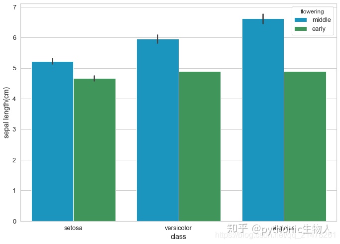
• 多重分类barplot

#按class分类后再按flowering分类barplot
plt.figure(dpi=70)
sns.set(style="whitegrid",font_scale=1.2)
sns.barplot(y='sepal length(cm)',x='class',data=pd_iris1,
              palette=["#01a2d9","#31A354","#c72e29"],
            hue='flowering'
             )

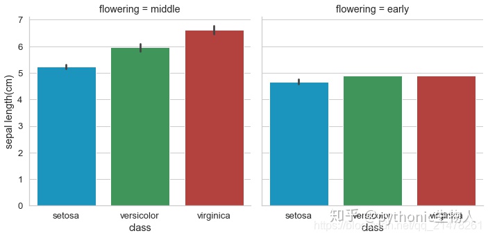
• ​catplot()结合 barplot()和FacetGrid绘制多子图

#使用catplot()结合 barplot()和FacetGrid分图显示
plt.figure(dpi=70)
sns.set(style="whitegrid",font_scale=1.2)
sns.catplot(y='sepal length(cm)',x='class',data=pd_iris1,
            palette=["#01a2d9","#31A354","#c72e29"],
            col='flowering',
            kind='bar',#
             )

---

9、seaborn.countplot

seaborn.countplot(x=None, y=None, hue=None, data=None, order=None, hue_order=None, orient=None, color=None, palette=None, saturation=0.75, dodge=True, ax=None, **kwargs)
简单理解为将数据去重，展现每个数据重复conuts数，非常类似barplot()

• 不分类countplot

#不分类countplot
plt.figure(dpi=90)
sns.set(style="whitegrid",font_scale=1.2)
sns.countplot(x='sepal length(cm)',data=pd_iris1,
              palette=["#1B813E","#E83015","#C1328E"], 
             )

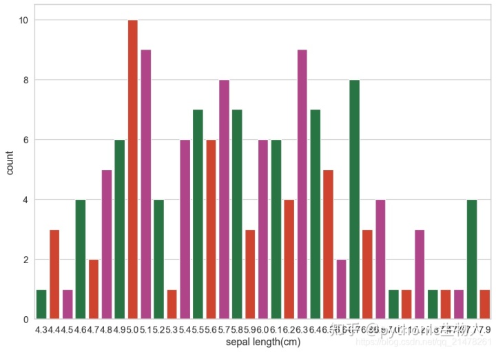
• 分类countplot

#分类countplot
plt.figure(dpi=90)
sns.set(style="whitegrid",font_scale=1.2)
sns.countplot(x='sepal length(cm)',data=pd_iris1,
              hue='class',#以上每个柱子在按class分三个柱子
              palette=["#1B813E","#E83015","#C1328E"], 
             )

• catplot()结合countplot和FacetGrid绘制多子图

#catplot()结合countplot和FacetGrid绘制多子图
#plt.figure(dpi=90)
sns.set(style="whitegrid",font_scale=1)
g=sns.catplot(x='sepal length(cm)',data=pd_iris1,
            hue='class',
            col='class',
            kind='count',#切换为countplot
            palette=["#1B813E","#E83015","#C1328E"], 
             )

参考资料

http://seaborn.pydata.org/generated/seaborn.catplot.html#seaborn.catplot

欢迎随缘关注@pythonic生物人