


一. 初始化参数:
- 1.1:使用0来初始化参数。
- 1.2:使用随机数来初始化参数。
- 1.3:使用抑梯度异常初始化参数(参见视频中的梯度消失和梯度爆炸)。
我们就开始导入相关的库:
import numpy as np
import matplotlib.pyplot as plt
import sklearn
import sklearn.datasets
from init_utils import sigmoid, relu, compute_loss, forward_propagation, backward_propagation
from init_utils import update_parameters, predict, load_dataset, plot_decision_boundary, predict_dec

%matplotlib inline
plt.rcParams['figure.figsize'] = (7.0, 4.0) # set default size of plots
plt.rcParams['image.interpolation'] = 'nearest'
plt.rcParams['image.cmap'] = 'gray'

# load image dataset: blue/red dots in circles
train_X, train_Y, test_X, test_Y = load_dataset()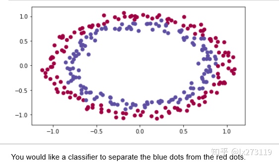
1 - Neural Network model
def model(X, Y, learning_rate = 0.01, num_iterations = 15000, print_cost = True, initialization = "he"):
"""
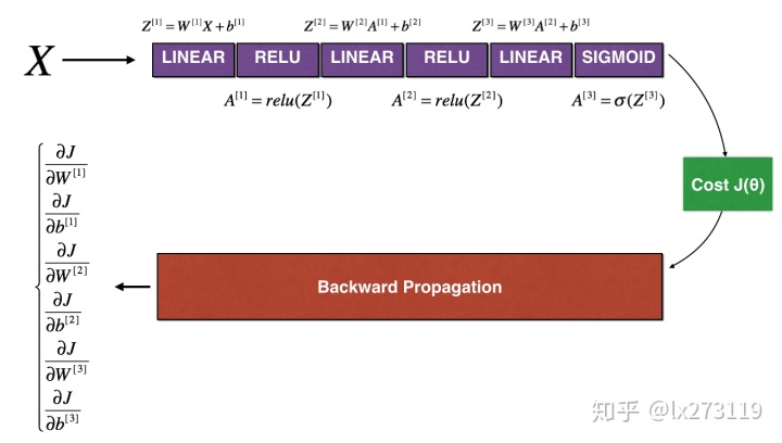
Implements a three-layer neural network: LINEAR->RELU->LINEAR->RELU->LINEAR->SIGMOID.
Arguments:
X -- input data, of shape (2, number of examples)
Y -- true "label" vector (containing 0 for red dots; 1 for blue dots), of shape (1, number of examples)
learning_rate -- learning rate for gradient descent
num_iterations -- number of iterations to run gradient descent
print_cost -- if True, print the cost every 1000 iterations
initialization -- flag to choose which initialization to use ("zeros","random" or "he")
Returns:
parameters -- parameters learnt by the model
"""
grads = {}
costs = [] # to keep track of the loss
m = X.shape[1] # number of examples
layers_dims = [X.shape[0], 10, 5, 1]
# Initialize parameters dictionary.
if initialization == "zeros":
parameters = initialize_parameters_zeros(layers_dims)
elif initialization == "random":
parameters = initialize_parameters_random(layers_dims)
elif initialization == "he":
parameters = initialize_parameters_he(layers_dims)
# Loop (gradient descent)
for i in range(0, num_iterations):
# Forward propagation: LINEAR -> RELU -> LINEAR -> RELU -> LINEAR -> SIGMOID.
a3, cache = forward_propagation(X, parameters)
# Loss
cost = compute_loss(a3, Y)
# Backward propagation.
grads = backward_propagation(X, Y, cache)
# Update parameters.
parameters = update_parameters(parameters, grads, learning_rate)
# Print the loss every 1000 iterations
if print_cost and i % 1000 == 0:
print("Cost after iteration {}: {}".format(i, cost))
costs.append(cost)
# plot the loss
plt.plot(costs)
plt.ylabel('cost')
plt.xlabel('iterations (per hundreds)')
plt.title("Learning rate =" + str(learning_rate))
plt.show()
return parameters2 - Zero initialization
def initialize_parameters_zeros(layers_dims):
    """
    Arguments:
    layer_dims -- python array (list) containing the size of each layer.

    Returns:
    parameters -- python dictionary containing your parameters "W1", "b1", ..., "WL", "bL":
                    W1 -- weight matrix of shape (layers_dims[1], layers_dims[0])
                    b1 -- bias vector of shape (layers_dims[1], 1)
                    ...
                    WL -- weight matrix of shape (layers_dims[L], layers_dims[L-1])
                    bL -- bias vector of shape (layers_dims[L], 1)
    """

    parameters = {}
    L = len(layers_dims)            # number of layers in the network

    for l in range(1, L):
        ### START CODE HERE ### (≈ 2 lines of code)
        parameters['W' + str(l)] = np.zeros((layers_dims[l],layers_dims[l-1]))
        parameters['b' + str(l)] = np.zeros((layers_dims[l],1))
        ### END CODE HERE ###
    return parameters
测试与结果:
parameters = initialize_parameters_zeros([3,2,1])
print("W1 = " + str(parameters["W1"]))
print("b1 = " + str(parameters["b1"]))
print("W2 = " + str(parameters["W2"]))
print("b2 = " + str(parameters["b2"]))- W1 = [[0. 0. 0.] [0. 0. 0.]]
- b1 = [[0.] [0.]]
- W2 = [[0. 0.]]
- b2 = [[0.]]
parameters = model(train_X, train_Y, initialization = "zeros")
print ("On the train set:")
predictions_train = predict(train_X, train_Y, parameters)
print ("On the test set:")
predictions_test = predict(test_X, test_Y, parameters)- Cost after iteration 0: 0.6931471805599453
- Cost after iteration 1000: 0.6931471805599453
- Cost after iteration 2000: 0.6931471805599453
- Cost after iteration 3000: 0.6931471805599453
- Cost after iteration 4000: 0.6931471805599453
- Cost after iteration 5000: 0.6931471805599453
- Cost after iteration 6000: 0.6931471805599453
- Cost after iteration 7000: 0.6931471805599453
- Cost after iteration 8000: 0.6931471805599453
- Cost after iteration 9000: 0.6931471805599453
- Cost after iteration 10000: 0.6931471805599455
- Cost after iteration 11000: 0.6931471805599453
- Cost after iteration 12000: 0.6931471805599453
- Cost after iteration 13000: 0.6931471805599453
- Cost after iteration 14000: 0.6931471805599453

print ("predictions_train = " + str(predictions_train))
print ("predictions_test = " + str(predictions_test))- predictions_train = [[0 0 0 0 0 0 0 0 0 0 0 0 0 0 0 0 0 0 0 0 0 0 0 0 0 0 0 0 0 0 0 0 0 0 0 0 0 0 0 0 0 0 0 0 0 0 0 0 0 0 0 0 0 0 0 0 0 0 0 0 0 0 0 0 0 0 0 0 0 0 0 0 0 0 0 0 0 0 0 0 0 0 0 0 0 0 0 0 0 0 0 0 0 0 0 0 0 0 0 0 0 0 0 0 0 0 0 0 0 0 0 0 0 0 0 0 0 0 0 0 0 0 0 0 0 0 0 0 0 0 0 0 0 0 0 0 0 0 0 0 0 0 0 0 0 0 0 0 0 0 0 0 0 0 0 0 0 0 0 0 0 0 0 0 0 0 0 0 0 0 0 0 0 0 0 0 0 0 0 0 0 0 0 0 0 0 0 0 0 0 0 0 0 0 0 0 0 0 0 0 0 0 0 0 0 0 0 0 0 0 0 0 0 0 0 0 0 0 0 0 0 0 0 0 0 0 0 0 0 0 0 0 0 0 0 0 0 0 0 0 0 0 0 0 0 0 0 0 0 0 0 0 0 0 0 0 0 0 0 0 0 0 0 0 0 0 0 0 0 0 0 0 0 0 0 0 0 0 0 0 0 0 0 0 0 0 0 0 0 0 0 0 0 0 0 0 0 0 0 0]]
- predictions_test = [[0 0 0 0 0 0 0 0 0 0 0 0 0 0 0 0 0 0 0 0 0 0 0 0 0 0 0 0 0 0 0 0 0 0 0 0 0 0 0 0 0 0 0 0 0 0 0 0 0 0 0 0 0 0 0 0 0 0 0 0 0 0 0 0 0 0 0 0 0 0 0 0 0 0 0 0 0 0 0 0 0 0 0 0 0 0 0 0 0 0 0 0 0 0 0 0 0 0 0 0]]
plt.title("Model with Zeros initialization")
axes = plt.gca()
axes.set_xlim([-1.5,1.5])
axes.set_ylim([-1.5,1.5])
plot_decision_boundary(lambda x: predict_dec(parameters, x.T), train_X, np.squeeze(train_Y))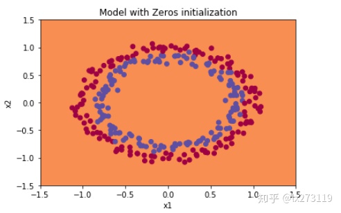
从上图中我们可以看到学习率一直没有变化,也就是说这个模型根本没有学习。分类失败,该模型预测每个都为0。通常来说,零初始化都会导致神经网络无法打破对称性,最终导致的结果就是无论网络有多少层,最终只能得到和Logistic函数相同的效果。
3 - Random initialization
#使用10倍缩放
def initialize_parameters_random(layers_dims):
    """
    Arguments:
    layer_dims -- python array (list) containing the size of each layer.

    Returns:
    parameters -- python dictionary containing your parameters "W1", "b1", ..., "WL", "bL":
                    W1 -- weight matrix of shape (layers_dims[1], layers_dims[0])
                    b1 -- bias vector of shape (layers_dims[1], 1)
                    ...
                    WL -- weight matrix of shape (layers_dims[L], layers_dims[L-1])
                    bL -- bias vector of shape (layers_dims[L], 1)
    """

    np.random.seed(3)               # This seed makes sure your "random" numbers will be the as ours
    parameters = {}
    L = len(layers_dims)            # integer representing the number of layers

    for l in range(1, L):
        ### START CODE HERE ### (≈ 2 lines of code)
        parameters['W' + str(l)] = np.random.randn(layers_dims[l],layers_dims[l-1])*10
        parameters['b' + str(l)] = np.zeros((layers_dims[l],1))
        ### END CODE HERE ###

    return parameters
测试与结果
parameters = initialize_parameters_random([3, 2, 1])
print("W1 = " + str(parameters["W1"]))
print("b1 = " + str(parameters["b1"]))
print("W2 = " + str(parameters["W2"]))
print("b2 = " + str(parameters["b2"]))
W1 = [[ 17.88628473 4.36509851 0.96497468] [-18.63492703 -2.77388203 -3.54758979]] b1 = [[0.] [0.]] W2 = [[-0.82741481 -6.27000677]] b2 = [[0.]]
parameters = model(train_X, train_Y, initialization = "random")
print ("On the train set:")
predictions_train = predict(train_X, train_Y, parameters)
print ("On the test set:")
predictions_test = predict(test_X, test_Y, parameters)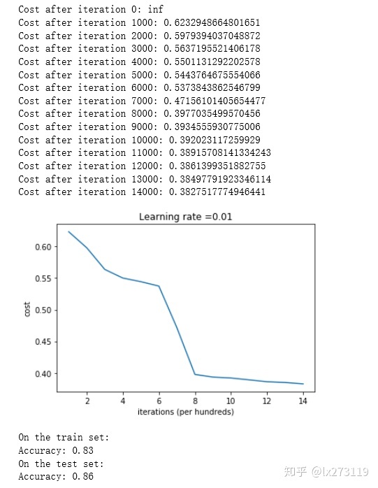
print (predictions_train)
print (predictions_test)- [[1 0 1 1 0 0 1 1 1 1 1 0 1 0 0 1 0 1 1 0 0 0 1 0 1 1 1 1 1 1 0 1 1 0 0 1 1 1 1 1 1 1 1 0 1 1 1 1 0 1 0 1 1 1 1 0 0 1 1 1 1 0 1 1 0 1 0 1 1 1 1 0 0 0 0 0 1 0 1 0 1 1 1 0 0 1 1 1 1 1 1 0 0 1 1 1 0 1 1 0 1 0 1 1 0 1 1 0 1 0 1 1 0 0 1 0 0 1 1 0 1 1 1 0 1 0 0 1 0 1 1 1 1 1 1 1 0 1 1 0 0 1 1 0 0 0 1 0 1 0 1 0 1 1 1 0 0 1 1 1 1 0 1 1 0 1 0 1 1 0 1 0 1 1 1 1 0 1 1 1 1 0 1 0 1 0 1 1 1 1 0 1 1 0 1 1 0 1 1 0 1 0 1 1 1 0 1 1 1 0 1 0 1 0 0 1 0 1 1 0 1 1 0 1 1 0 1 1 1 0 1 1 1 1 0 1 0 0 1 1 0 1 1 1 0 0 0 1 1 0 1 1 1 1 0 1 1 0 1 1 1 0 0 1 0 0 0 1 0 0 0 1 1 1 1 0 0 0 0 1 1 1 1 0 0 1 1 1 1 1 1 1 0 0 0 1 1 1 1 0]]
- [[1 1 1 1 0 1 0 1 1 0 1 1 1 0 0 0 0 1 0 1 0 0 1 0 1 0 1 1 1 1 1 0 0 0 0 1 0 1 1 0 0 1 1 1 1 1 0 1 1 1 0 1 0 1 1 0 1 0 1 0 1 1 1 1 1 1 1 1 1 0 1 0 1 1 1 1 1 0 1 0 0 1 0 0 0 1 1 0 1 1 0 0 0 1 1 0 1 1 0 0]]
plt.title("Model with large random initialization")
axes = plt.gca()
axes.set_xlim([-1.5,1.5])
axes.set_ylim([-1.5,1.5])
plot_decision_boundary(lambda x: predict_dec(parameters, x.T), train_X, np.squeeze(train_Y))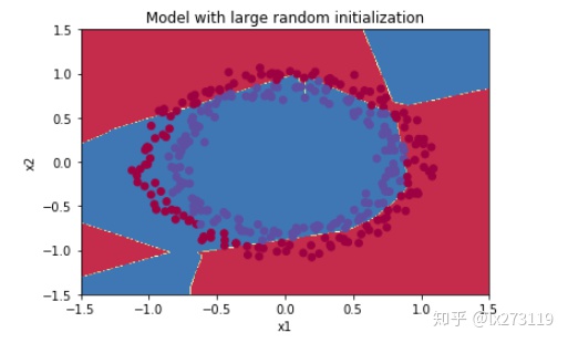
我们可以看到误差开始很高。这是因为由于具有较大的随机权重,最后一个激活(sigmoid)输出的结果非常接近于0或1,而当它出现错误时,它会导致非常高的损失。初始化参数如果没有很好地话会导致梯度消失、爆炸,这也会减慢优化算法。如果我们对这个网络进行更长时间的训练,我们将看到更好的结果,但是使用过大的随机数初始化会减慢优化的速度。
总而言之,将权重初始化为非常大的时候其实效果并不好,下面我们试试小一点的参数值。
4 - He initialization
def initialize_parameters_he(layers_dims):
    """
    Arguments:
    layer_dims -- python array (list) containing the size of each layer.

    Returns:
    parameters -- python dictionary containing your parameters "W1", "b1", ..., "WL", "bL":
                    W1 -- weight matrix of shape (layers_dims[1], layers_dims[0])
                    b1 -- bias vector of shape (layers_dims[1], 1)
                    ...
                    WL -- weight matrix of shape (layers_dims[L], layers_dims[L-1])
                    bL -- bias vector of shape (layers_dims[L], 1)
    """

    np.random.seed(3)
    parameters = {}
    L = len(layers_dims) - 1 # integer representing the number of layers

    for l in range(1, L + 1):
        ### START CODE HERE ### (≈ 2 lines of code)
        parameters['W' + str(l)] = np.random.randn(layers_dims[l],layers_dims[l-1])*np.sqrt(2/layers_dims[l-1])
        parameters['b' + str(l)] = np.zeros((layers_dims[l],1))*np.sqrt(2/layers_dims[l-1])
        ### END CODE HERE ###

    return parameters
测试and结果
parameters = initialize_parameters_he([2, 4, 1])
print("W1 = " + str(parameters["W1"]))
print("b1 = " + str(parameters["b1"]))
print("W2 = " + str(parameters["W2"]))
print("b2 = " + str(parameters["b2"]))
W1 = [[ 1.78862847 0.43650985] [ 0.09649747 -1.8634927 ] [-0.2773882 -0.35475898] [-0.08274148 -0.62700068]] b1 = [[0.] [0.] [0.] [0.]] W2 = [[-0.03098412 -0.33744411 -0.92904268 0.62552248]] b2 = [[0.]]

plt.title("Model with He initialization")
axes = plt.gca()
axes.set_xlim([-1.5,1.5])
axes.set_ylim([-1.5,1.5])
plot_decision_boundary(lambda x: predict_dec(parameters, x.T), train_X, np.squeeze(train_Y))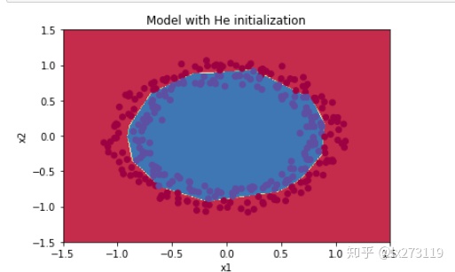
初始化的模型将蓝色和红色的点在少量的迭代中很好地分离出来,
总结一下:
- 不同的初始化方法可能导致性能最终不同
- 随机初始化有助于打破对称,使得不同隐藏层的单元可以学习到不同的参数。
- 初始化时,初始值不宜过大。
- He初始化搭配ReLU激活函数常常可以得到不错的效果。
二. 正则化
在深度学习中,如果数据集没有足够大的话,可能会导致一些过拟合的问题。过拟合导致的结果就是在训练集上有着很高的精确度,但是在遇到新的样本时,精确度下降会很严重。为了避免过拟合的问题,接下来我们要讲解的方式就是正则化。
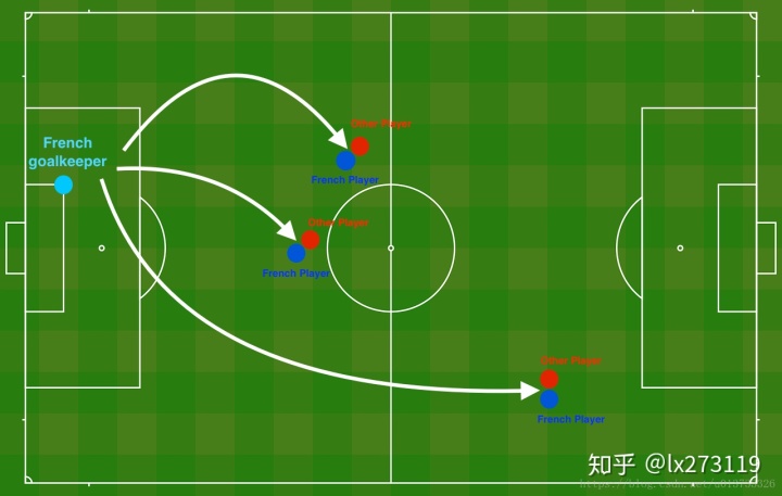
问题描述:假设你现在是一个AI专家,你需要设计一个模型,可以用于推荐在足球场中守门员将球发至哪个位置可以让本队的球员抢到球的可能性更大。说白了,实际上就是一个二分类,一半是己方抢到球,一半就是对方抢到球,我们来看一下这个图:
读取并绘制数据集
我们来加载并查看一下我们的数据集:
train_X, train_Y, test_X, test_Y = load_2D_dataset()
每一个点代表球落下的可能的位置,蓝色代表己方的球员会抢到球,红色代表对手的球员会抢到球,我们要做的就是使用模型来画出一条线,来找到适合我方球员能抢到球的位置。
我们要做以下三件事,来对比出不同的模型的优劣:
不使用正则化
使用正则化
2.1 使用L2正则化
2.2 使用随机节点删除
def model(X, Y, learning_rate = 0.3, num_iterations = 30000, print_cost = True, lambd = 0, keep_prob = 1):
    """
    Implements a three-layer neural network: LINEAR->RELU->LINEAR->RELU->LINEAR->SIGMOID.

    Arguments:
    X -- input data, of shape (input size, number of examples)
    Y -- true "label" vector (1 for blue dot / 0 for red dot), of shape (output size, number of examples)
    learning_rate -- learning rate of the optimization
    num_iterations -- number of iterations of the optimization loop
    print_cost -- If True, print the cost every 10000 iterations
    lambd -- regularization hyperparameter, scalar
    keep_prob - probability of keeping a neuron active during drop-out, scalar.

    Returns:
    parameters -- parameters learned by the model. They can then be used to predict.
    """

    grads = {}
    costs = []                            # to keep track of the cost
    m = X.shape[1]                        # number of examples
    layers_dims = [X.shape[0], 20, 3, 1]

    # Initialize parameters dictionary.
    parameters = initialize_parameters(layers_dims)

    # Loop (gradient descent)

    for i in range(0, num_iterations):

        # Forward propagation: LINEAR -> RELU -> LINEAR -> RELU -> LINEAR -> SIGMOID.
        if keep_prob == 1:
            a3, cache = forward_propagation(X, parameters)
        elif keep_prob < 1:
            a3, cache = forward_propagation_with_dropout(X, parameters, keep_prob)

        # Cost function
        if lambd == 0:
            cost = compute_cost(a3, Y)
        else:
            cost = compute_cost_with_regularization(a3, Y, parameters, lambd)

        # Backward propagation.
        assert(lambd==0 or keep_prob==1)    # it is possible to use both L2 regularization and dropout,
                                            # but this assignment will only explore one at a time
        if lambd == 0 and keep_prob == 1:
            grads = backward_propagation(X, Y, cache)
        elif lambd != 0:
            grads = backward_propagation_with_regularization(X, Y, cache, lambd)
        elif keep_prob < 1:
            grads = backward_propagation_with_dropout(X, Y, cache, keep_prob)

        # Update parameters.
        parameters = update_parameters(parameters, grads, learning_rate)

        # Print the loss every 10000 iterations
        if print_cost and i % 10000 == 0:
            print("Cost after iteration {}: {}".format(i, cost))
        if print_cost and i % 1000 == 0:
            costs.append(cost)

    # plot the cost
    plt.plot(costs)
    plt.ylabel('cost')
    plt.xlabel('iterations (x1,000)')
    plt.title("Learning rate =" + str(learning_rate))
    plt.show()

    return parameters
Let's train the model without any regularization, and observe the accuracy on the train/test sets.
parameters = model(train_X, train_Y)
print ("On the training set:")
predictions_train = predict(train_X, train_Y, parameters)
print ("On the test set:")
predictions_test = predict(test_X, test_Y, parameters)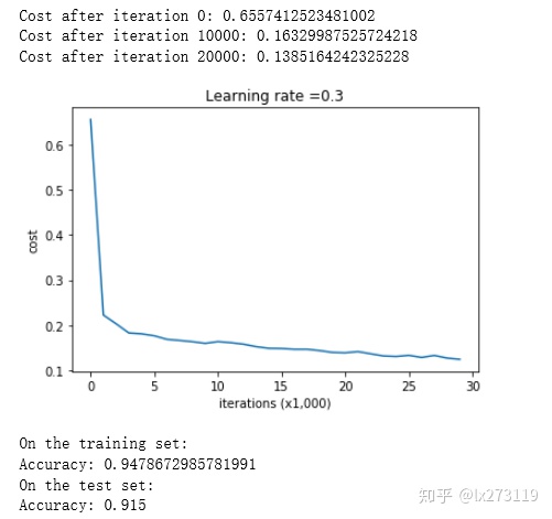
对于训练集,精确度为94%;而对于测试集,精确度为91.5%。接下来,我们将分割曲线画出来:
plt.title("Model without regularization")
axes = plt.gca()
axes.set_xlim([-0.75,0.40])
axes.set_ylim([-0.75,0.65])
plot_decision_boundary(lambda x: predict_dec(parameters, x.T), train_X, np.squeeze(train_Y))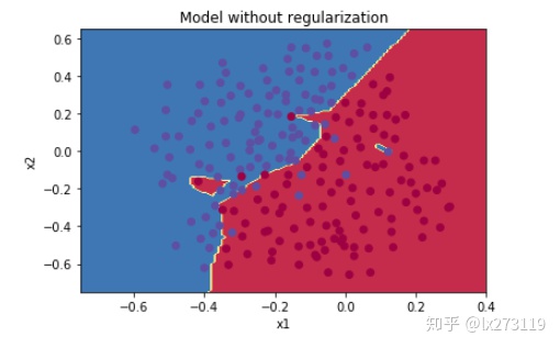
2 - L2 Regularization

# GRADED FUNCTION: compute_cost_with_regularization

def compute_cost_with_regularization(A3, Y, parameters, lambd):
    """
    Implement the cost function with L2 regularization. See formula (2) above.

    Arguments:
    A3 -- post-activation, output of forward propagation, of shape (output size, number of examples)
    Y -- "true" labels vector, of shape (output size, number of examples)
    parameters -- python dictionary containing parameters of the model

    Returns:
    cost - value of the regularized loss function (formula (2))
    """
    m = Y.shape[1]
    W1 = parameters["W1"]
    W2 = parameters["W2"]
    W3 = parameters["W3"]

    cross_entropy_cost = compute_cost(A3, Y) # This gives you the cross-entropy part of the cost

    ### START CODE HERE ### (approx. 1 line)
    L2_regularization_cost = lambd/(2*m)*(np.sum(np.square(W1))+np.sum(np.square(W2))+np.sum(np.square(W3)))
    ### END CODER HERE ###

    cost = cross_entropy_cost + L2_regularization_cost

    return cost
检验和结果
A3, Y_assess, parameters = compute_cost_with_regularization_test_case()

print("cost = " + str(compute_cost_with_regularization(A3, Y_assess, parameters, lambd = 0.1)))
cost = 1.7864859451590758
def backward_propagation_with_regularization(X, Y, cache, lambd):
    """
    Implements the backward propagation of our baseline model to which we added an L2 regularization.

    Arguments:
    X -- input dataset, of shape (input size, number of examples)
    Y -- "true" labels vector, of shape (output size, number of examples)
    cache -- cache output from forward_propagation()
    lambd -- regularization hyperparameter, scalar

    Returns:
    gradients -- A dictionary with the gradients with respect to each parameter, activation and pre-activation variables
    """

    m = X.shape[1]
    (Z1, A1, W1, b1, Z2, A2, W2, b2, Z3, A3, W3, b3) = cache

    dZ3 = A3 - Y

    ### START CODE HERE ### (approx. 1 line)
    dW3 = 1./m * np.dot(dZ3, A2.T) + lambd*W3/m
    ### END CODE HERE ###
    db3 = 1./m * np.sum(dZ3, axis=1, keepdims = True)

    dA2 = np.dot(W3.T, dZ3)
    dZ2 = np.multiply(dA2, np.int64(A2 > 0))
    ### START CODE HERE ### (approx. 1 line)
    dW2 = 1./m * np.dot(dZ2, A1.T) + lambd*W2/m
    ### END CODE HERE ###
    db2 = 1./m * np.sum(dZ2, axis=1, keepdims = True)

    dA1 = np.dot(W2.T, dZ2)
    dZ1 = np.multiply(dA1, np.int64(A1 > 0))
    ### START CODE HERE ### (approx. 1 line)
    dW1 = 1./m * np.dot(dZ1, X.T) + lambd*W1/m
    ### END CODE HERE ###
    db1 = 1./m * np.sum(dZ1, axis=1, keepdims = True)

    gradients = {"dZ3": dZ3, "dW3": dW3, "db3": db3,"dA2": dA2,
                 "dZ2": dZ2, "dW2": dW2, "db2": db2, "dA1": dA1,
                 "dZ1": dZ1, "dW1": dW1, "db1": db1}

    return gradients
测试和结果
X_assess, Y_assess, cache = backward_propagation_with_regularization_test_case()

grads = backward_propagation_with_regularization(X_assess, Y_assess, cache, lambd = 0.7)
print ("dW1 = "+ str(grads["dW1"]))
print ("dW2 = "+ str(grads["dW2"]))
print ("dW3 = "+ str(grads["dW3"]))
dW1 = [[-0.25604646 0.12298827 -0.28297129] [-0.17706303 0.34536094 -0.4410571 ]] dW2 = [[ 0.79276486 0.85133918] [-0.0957219 -0.01720463] [-0.13100772 -0.03750433]] dW3 = [[-1.77691347 -0.11832879 -0.09397446]]
Let's now run the model with L2 regularization ( =0.7)
parameters = model(train_X, train_Y, lambd = 0.7)
print ("On the train set:")
predictions_train = predict(train_X, train_Y, parameters)
print ("On the test set:")
predictions_test = predict(test_X, test_Y, parameters)
Let's plot the decision boundary.
plt.title("Model with L2-regularization")
axes = plt.gca()
axes.set_xlim([-0.75,0.40])
axes.set_ylim([-0.75,0.65])
plot_decision_boundary(lambda x: predict_dec(parameters, x.T), train_X, np.squeeze(train_Y))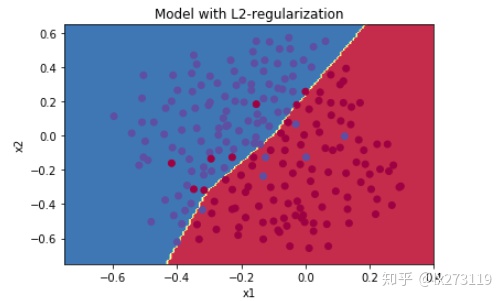
λ的值是可以使用开发集调整时的超参数。L2正则化会使决策边界更加平滑。如果λ太大,也可能会“过度平滑”,从而导致模型高偏差。L2正则化实际上在做什么?L2正则化依赖于较小权重的模型比具有较大权重的模型更简单这样的假设,因此,通过削减成本函数中权重的平方值,可以将所有权重值逐渐改变到到较小的值。权值数值高的话会有更平滑的模型,其中输入变化时输出变化更慢,但是你需要花费更多的时间。L2正则化对以下内容有影响:
成本计算: 正则化的计算需要添加到成本函数中
反向传播功能:在权重矩阵方面,梯度计算时也要依据正则化来做出相应的计算
重量变小(“重量衰减”):权重被逐渐改变到较小的值。
3 - Dropout
3.1 - Forward propagation with dropout
def forward_propagation_with_dropout(X, parameters, keep_prob = 0.5):
    """
    Implements the forward propagation: LINEAR -> RELU + DROPOUT -> LINEAR -> RELU + DROPOUT -> LINEAR -> SIGMOID.

    Arguments:
    X -- input dataset, of shape (2, number of examples)
    parameters -- python dictionary containing your parameters "W1", "b1", "W2", "b2", "W3", "b3":
                    W1 -- weight matrix of shape (20, 2)
                    b1 -- bias vector of shape (20, 1)
                    W2 -- weight matrix of shape (3, 20)
                    b2 -- bias vector of shape (3, 1)
                    W3 -- weight matrix of shape (1, 3)
                    b3 -- bias vector of shape (1, 1)
    keep_prob - probability of keeping a neuron active during drop-out, scalar

    Returns:
    A3 -- last activation value, output of the forward propagation, of shape (1,1)
    cache -- tuple, information stored for computing the backward propagation
    """

    np.random.seed(1)

    # retrieve parameters
    W1 = parameters["W1"]
    b1 = parameters["b1"]
    W2 = parameters["W2"]
    b2 = parameters["b2"]
    W3 = parameters["W3"]
    b3 = parameters["b3"]

    # LINEAR -> RELU -> LINEAR -> RELU -> LINEAR -> SIGMOID
    Z1 = np.dot(W1, X) + b1
    A1 = relu(Z1)
    ### START CODE HERE ### (approx. 4 lines)         # Steps 1-4 below correspond to the Steps 1-4 described above.
    D1 = np.random.rand(A1.shape[0],A1.shape[1])                                         # Step 1: initialize matrix D1 = np.random.rand(..., ...)
    D1 = D1 < keep_prob                                       # Step 2: convert entries of D1 to 0 or 1 (using keep_prob as the threshold)
    A1 = np.multiply(D1,A1)                                         # Step 3: shut down some neurons of A1
    A1 = A1/keep_prob                                        # Step 4: scale the value of neurons that haven't been shut down
    ### END CODE HERE ###
    Z2 = np.dot(W2, A1) + b2
    A2 = relu(Z2)
    ### START CODE HERE ### (approx. 4 lines)
    D2 = np.random.rand(A2.shape[0],A2.shape[1])                                         # Step 1: initialize matrix D2 = np.random.rand(..., ...)
    D2 = D2 < keep_prob                                         # Step 2: convert entries of D2 to 0 or 1 (using keep_prob as the threshold)
    A2 = np.multiply(D2,A2)                                         # Step 3: shut down some neurons of A2
    A2 = A2/keep_prob                                        # Step 4: scale the value of neurons that haven't been shut down
    ### END CODE HERE ###
    Z3 = np.dot(W3, A2) + b3
    A3 = sigmoid(Z3)

    cache = (Z1, D1, A1, W1, b1, Z2, D2, A2, W2, b2, Z3, A3, W3, b3)

    return A3, cache
检测与结果
X_assess, parameters = forward_propagation_with_dropout_test_case()

A3, cache = forward_propagation_with_dropout(X_assess, parameters, keep_prob = 0.7)
print ("A3 = " + str(A3))
A3 = [[0.36974721 0.00305176 0.04565099 0.49683389 0.36974721]]
3.2 - Backward propagation with dropout
# GRADED FUNCTION: backward_propagation_with_dropout

def backward_propagation_with_dropout(X, Y, cache, keep_prob):
    """
    Implements the backward propagation of our baseline model to which we added dropout.

    Arguments:
    X -- input dataset, of shape (2, number of examples)
    Y -- "true" labels vector, of shape (output size, number of examples)
    cache -- cache output from forward_propagation_with_dropout()
    keep_prob - probability of keeping a neuron active during drop-out, scalar

    Returns:
    gradients -- A dictionary with the gradients with respect to each parameter, activation and pre-activation variables
    """

    m = X.shape[1]
    (Z1, D1, A1, W1, b1, Z2, D2, A2, W2, b2, Z3, A3, W3, b3) = cache

    dZ3 = A3 - Y
    dW3 = 1./m * np.dot(dZ3, A2.T)
    db3 = 1./m * np.sum(dZ3, axis=1, keepdims = True)
    dA2 = np.dot(W3.T, dZ3)
    ### START CODE HERE ### (≈ 2 lines of code)
    dA2 = dA2 * D2           # Step 1: Apply mask D2 to shut down the same neurons as during the forward propagation
    dA2 = dA2/keep_prob              # Step 2: Scale the value of neurons that haven't been shut down
    ### END CODE HERE ###
    dZ2 = np.multiply(dA2, np.int64(A2 > 0))
    dW2 = 1./m * np.dot(dZ2, A1.T)
    db2 = 1./m * np.sum(dZ2, axis=1, keepdims = True)

    dA1 = np.dot(W2.T, dZ2)
    ### START CODE HERE ### (≈ 2 lines of code)
    dA1 = dA1 *D1              # Step 1: Apply mask D1 to shut down the same neurons as during the forward propagation
    dA1 = dA1/keep_prob           # Step 2: Scale the value of neurons that haven't been shut down
    ### END CODE HERE ###
    dZ1 = np.multiply(dA1, np.int64(A1 > 0))
    dW1 = 1./m * np.dot(dZ1, X.T)
    db1 = 1./m * np.sum(dZ1, axis=1, keepdims = True)

    gradients = {"dZ3": dZ3, "dW3": dW3, "db3": db3,"dA2": dA2,
                 "dZ2": dZ2, "dW2": dW2, "db2": db2, "dA1": dA1,
                 "dZ1": dZ1, "dW1": dW1, "db1": db1}

    return gradients
检验与结果
X_assess, Y_assess, cache = backward_propagation_with_dropout_test_case()

gradients = backward_propagation_with_dropout(X_assess, Y_assess, cache, keep_prob = 0.8)

print ("dA1 = " + str(gradients["dA1"]))
print ("dA2 = " + str(gradients["dA2"]))
dA1 = [[ 0.36544439 0. -0.00188233 0. -0.17408748] [ 0.65515713 0. -0.00337459 0. -0. ]] dA2 = [[ 0.58180856 0. -0.00299679 0. -0.27715731] [ 0. 0.53159854 -0. 0.53159854 -0.34089673] [ 0. 0. -0.00292733 0. -0. ]]
现在用dropout运行模型
parameters = model(train_X, train_Y, keep_prob = 0.86, learning_rate = 0.3)

print ("On the train set:")
predictions_train = predict(train_X, train_Y, parameters)
print ("On the test set:")
predictions_test = predict(test_X, test_Y, parameters)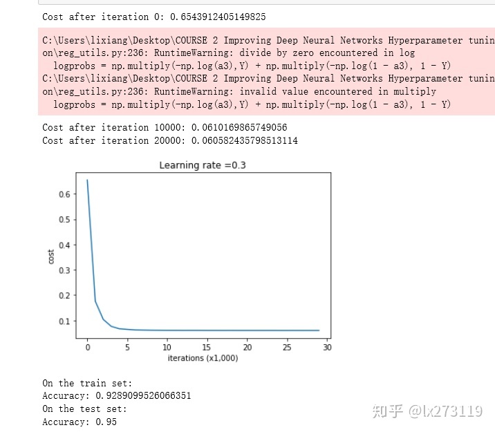
plt.title("Model with dropout")
axes = plt.gca()
axes.set_xlim([-0.75,0.40])
axes.set_ylim([-0.75,0.65])
plot_decision_boundary(lambda x: predict_dec(parameters, x.T), train_X, np.squeeze(train_Y))
我们可以看到,正则化会把训练集的准确度降低,但是测试集的准确度提高了,所以,我们这个还是成功了。
三. 梯度检验
让我们回头看一下导数(或梯度)的定义:
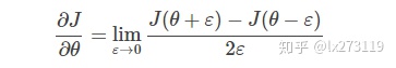
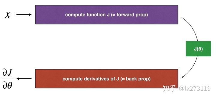
def forward_propagation(x, theta):
    """
    Implement the linear forward propagation (compute J) presented in Figure 1 (J(theta) = theta * x)

    Arguments:
    x -- a real-valued input
    theta -- our parameter, a real number as well

    Returns:
    J -- the value of function J, computed using the formula J(theta) = theta * x
    """

    ### START CODE HERE ### (approx. 1 line)
    J = theta * x
    ### END CODE HERE ###

    return J
检验与结果
x, theta = 2, 4
J = forward_propagation(x, theta)
print ("J = " + str(J))
J = 8
def backward_propagation(x, theta):
    """
    Computes the derivative of J with respect to theta (see Figure 1).

    Arguments:
    x -- a real-valued input
    theta -- our parameter, a real number as well

    Returns:
    dtheta -- the gradient of the cost with respect to theta
    """

    ### START CODE HERE ### (approx. 1 line)
    dtheta = x
    ### END CODE HERE ###

    return dtheta
检验与结果
x, theta = 2, 4
dtheta = backward_propagation(x, theta)
print ("dtheta = " + str(dtheta))
dtheta = 2
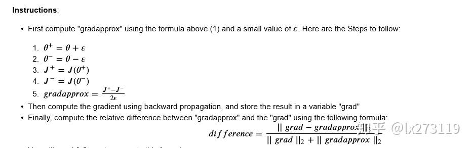
# GRADED FUNCTION: gradient_check

def gradient_check(x, theta, epsilon = 1e-7):
    """
    Implement the backward propagation presented in Figure 1.

    Arguments:
    x -- a real-valued input
    theta -- our parameter, a real number as well
    epsilon -- tiny shift to the input to compute approximated gradient with formula(1)

    Returns:
    difference -- difference (2) between the approximated gradient and the backward propagation gradient
    """

    # Compute gradapprox using left side of formula (1). epsilon is small enough, you don't need to worry about the limit.
    ### START CODE HERE ### (approx. 5 lines)
    thetaplus = theta + epsilon                              # Step 1
    thetaminus = theta - epsilon                             # Step 2
    J_plus = forward_propagation(x,thetaplus)                                 # Step 3
    J_minus = forward_propagation(x,thetaminus)                                # Step 4
    gradapprox = (J_plus- J_minus)/(2*epsilon )                           # Step 5
    ### END CODE HERE ###

    # Check if gradapprox is close enough to the output of backward_propagation()
    ### START CODE HERE ### (approx. 1 line)
    grad = backward_propagation(x,theta)
    ### END CODE HERE ###

    ### START CODE HERE ### (approx. 1 line)
    numerator = np.linalg.norm(gradapprox-grad)                             # Step 1'
    denominator = np.linalg.norm(gradapprox)+np.linalg.norm(grad)                              # Step 2'
    difference = numerator/  denominator                            # Step 3'
    ### END CODE HERE ###

    if difference < 1e-7:
        print ("The gradient is correct!")
    else:
        print ("The gradient is wrong!")

    return difference
测试一下:
#测试gradient_check
print("-----------------测试gradient_check-----------------")
x, theta = 2, 4
difference = gradient_check(x, theta)
print("difference = " + str(difference))
结果:
The gradient is correct! difference = 2.919335883291695e-10
3) N-dimensional gradient checking
def forward_propagation_n(X, Y, parameters):
    """
    Implements the forward propagation (and computes the cost) presented in Figure 3.

    Arguments:
    X -- training set for m examples
    Y -- labels for m examples
    parameters -- python dictionary containing your parameters "W1", "b1", "W2", "b2", "W3", "b3":
                    W1 -- weight matrix of shape (5, 4)
                    b1 -- bias vector of shape (5, 1)
                    W2 -- weight matrix of shape (3, 5)
                    b2 -- bias vector of shape (3, 1)
                    W3 -- weight matrix of shape (1, 3)
                    b3 -- bias vector of shape (1, 1)

    Returns:
    cost -- the cost function (logistic cost for one example)
    """

    # retrieve parameters
    m = X.shape[1]
    W1 = parameters["W1"]
    b1 = parameters["b1"]
    W2 = parameters["W2"]
    b2 = parameters["b2"]
    W3 = parameters["W3"]
    b3 = parameters["b3"]

    # LINEAR -> RELU -> LINEAR -> RELU -> LINEAR -> SIGMOID
    Z1 = np.dot(W1, X) + b1
    A1 = relu(Z1)
    Z2 = np.dot(W2, A1) + b2
    A2 = relu(Z2)
    Z3 = np.dot(W3, A2) + b3
    A3 = sigmoid(Z3)

    # Cost
    logprobs = np.multiply(-np.log(A3),Y) + np.multiply(-np.log(1 - A3), 1 - Y)
    cost = 1./m * np.sum(logprobs)

    cache = (Z1, A1, W1, b1, Z2, A2, W2, b2, Z3, A3, W3, b3)

    return cost, cache
Now, run backward propagation
def backward_propagation_n(X, Y, cache):
    """
    Implement the backward propagation presented in figure 2.

    Arguments:
    X -- input datapoint, of shape (input size, 1)
    Y -- true "label"
    cache -- cache output from forward_propagation_n()

    Returns:
    gradients -- A dictionary with the gradients of the cost with respect to each parameter, activation and pre-activation variables.
    """

    m = X.shape[1]
    (Z1, A1, W1, b1, Z2, A2, W2, b2, Z3, A3, W3, b3) = cache

    dZ3 = A3 - Y
    dW3 = 1./m * np.dot(dZ3, A2.T)
    db3 = 1./m * np.sum(dZ3, axis=1, keepdims = True)

    dA2 = np.dot(W3.T, dZ3)
    dZ2 = np.multiply(dA2, np.int64(A2 > 0))
    dW2 = 1./m * np.dot(dZ2, A1.T) * 2
    db2 = 1./m * np.sum(dZ2, axis=1, keepdims = True)

    dA1 = np.dot(W2.T, dZ2)
    dZ1 = np.multiply(dA1, np.int64(A1 > 0))
    dW1 = 1./m * np.dot(dZ1, X.T)
    db1 = 4./m * np.sum(dZ1, axis=1, keepdims = True)

    gradients = {"dZ3": dZ3, "dW3": dW3, "db3": db3,
                 "dA2": dA2, "dZ2": dZ2, "dW2": dW2, "db2": db2,
                 "dA1": dA1, "dZ1": dZ1, "dW1": dW1, "db1": db1}

    return gradients
这个代码中是有错误的地方,可以检验一下,现在检验
# GRADED FUNCTION: gradient_check_n

def gradient_check_n(parameters, gradients, X, Y, epsilon = 1e-7):
    """
    Checks if backward_propagation_n computes correctly the gradient of the cost output by forward_propagation_n

    Arguments:
    parameters -- python dictionary containing your parameters "W1", "b1", "W2", "b2", "W3", "b3":
    grad -- output of backward_propagation_n, contains gradients of the cost with respect to the parameters.
    x -- input datapoint, of shape (input size, 1)
    y -- true "label"
    epsilon -- tiny shift to the input to compute approximated gradient with formula(1)

    Returns:
    difference -- difference (2) between the approximated gradient and the backward propagation gradient
    """

    # Set-up variables
    parameters_values, _ = dictionary_to_vector(parameters)
    grad = gradients_to_vector(gradients)
    num_parameters = parameters_values.shape[0]
    J_plus = np.zeros((num_parameters, 1))
    J_minus = np.zeros((num_parameters, 1))
    gradapprox = np.zeros((num_parameters, 1))

    # Compute gradapprox
    for i in range(num_parameters):

        # Compute J_plus[i]. Inputs: "parameters_values, epsilon". Output = "J_plus[i]".
        # "_" is used because the function you have to outputs two parameters but we only care about the first one
        ### START CODE HERE ### (approx. 3 lines)
        thetaplus =  np.copy(parameters_values)                                  # Step 1
        thetaplus[i][0] =  thetaplus[i][0] + epsilon                              # Step 2
        J_plus[i], cache = forward_propagation_n(X,Y,vector_to_dictionary(thetaplus))                                   # Step 3
        ### END CODE HERE ###

        # Compute J_minus[i]. Inputs: "parameters_values, epsilon". Output = "J_minus[i]".
        ### START CODE HERE ### (approx. 3 lines)
        thetaminus = np.copy(parameters_values)                                   # Step 1
        thetaminus[i][0] =  thetaminus[i][0] - epsilon                            # Step 2
        J_minus[i], cache =  forward_propagation_n(X,Y,vector_to_dictionary(thetaminus))                               # Step 3
        ### END CODE HERE ###

        # Compute gradapprox[i]
        ### START CODE HERE ### (approx. 1 line)
        gradapprox[i] = (J_plus[i] - J_minus[i])/(2*epsilon)
        ### END CODE HERE ###

    # Compare gradapprox to backward propagation gradients by computing difference.
    ### START CODE HERE ### (approx. 1 line)
    numerator = np.linalg.norm(grad-gradapprox)                                          # Step 1'
    denominator = np.linalg.norm(grad)+   np.linalg.norm(gradapprox)                                      # Step 2'
    difference = numerator /  denominator                                        # Step 3'
    ### END CODE HERE ###

    if difference > 1e-7:
        print ("033[93m" + "There is a mistake in the backward propagation! difference = " + str(difference) + "033[0m")
    else:
        print ("033[92m" + "Your backward propagation works perfectly fine! difference = " + str(difference) + "033[0m")

    return difference
检验:
X, Y, parameters = gradient_check_n_test_case()

cost, cache = forward_propagation_n(X, Y, parameters)
gradients = backward_propagation_n(X, Y, cache)
difference = gradient_check_n(parameters, gradients, X, Y)
There is a mistake in the backward propagation! difference = 0.285093156780699
backward_propagation_n(X, Y, cache)函数中,2处出现错误。
dW2 = 1./m * np.dot(dZ2, A1.T) * 2
db1 = 4./m * np.sum(dZ1, axis=1, keepdims = True)


 8万+
8万+


 被折叠的 条评论
为什么被折叠?
被折叠的 条评论
为什么被折叠?
 到【灌水乐园】发言


