


引言:
TensorFlow是一个采用数据流图(data flow graphs),用于数值计算的开源软件库。其在机器学习和深度学习中具有广泛的应用,掌握TF无疑对于机器学习的理解是很有帮助的。有时候,只看还是略显肤浅,亲自调试代码才能学 的更多。
自己以前并未意识到TF的重要性,值得好好研究
重要参考资料:
TensorFlow Examples - TensorFlow tutorials and code examples for beginners TensorFlow-Course https:// github.com/machinelearn ingmindset/TensorFlow-Course

TensorFlow的设计理念体现在以下方面:
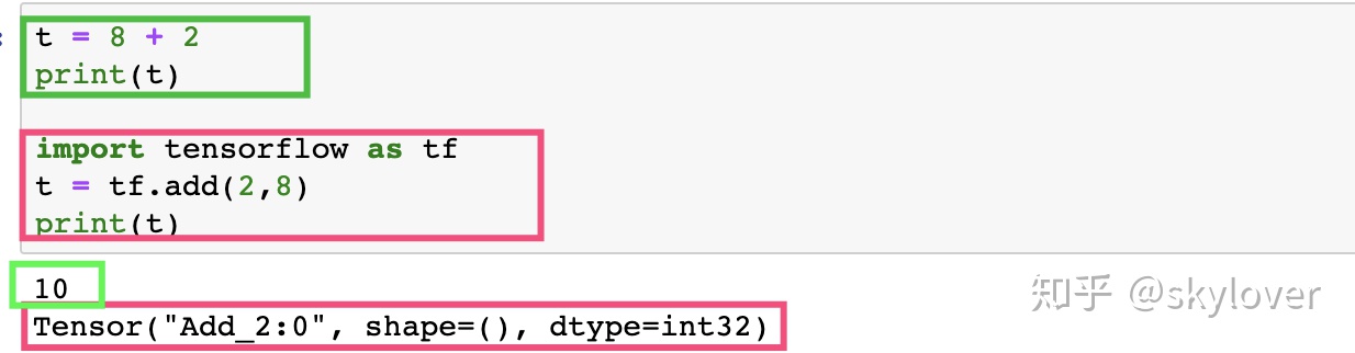
将图的定义和图的运行完全分开,因此TensorFlow被认为 是一个“符号主义”的库,采用符号式编程。
传统的命令式编程如下:
t = 8 + 2
print(t)
上述命令定义了t 的运算,在运行时就执行了,并输出 10
而在TensorFlow 中,并未执行:
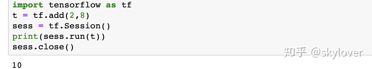
而图的运行必须放在会话(session)中。
开启会话后,就可以用数据填充节点,进行计算
关闭会话,则计算结束
顾名思义,TensorFlow 意思是“张量的流动”,数据流图如下:
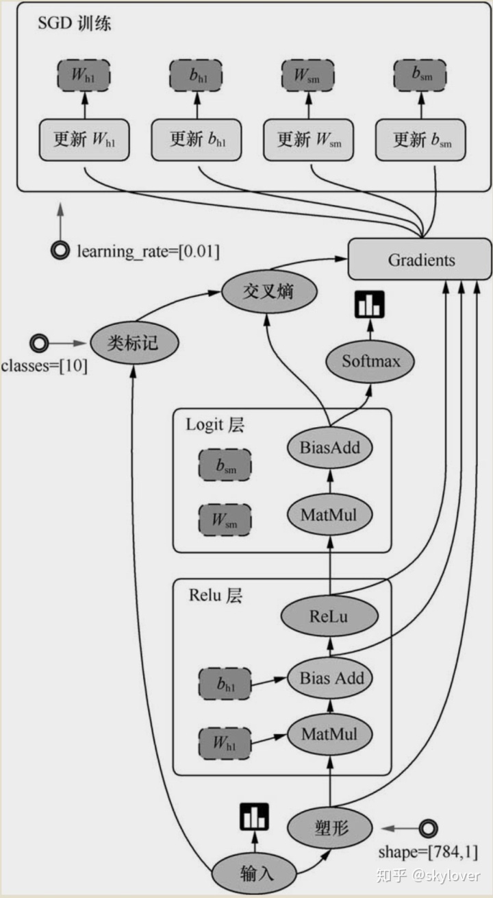
关于Logit 层,参见[1]
TensorFlow 源代码学习
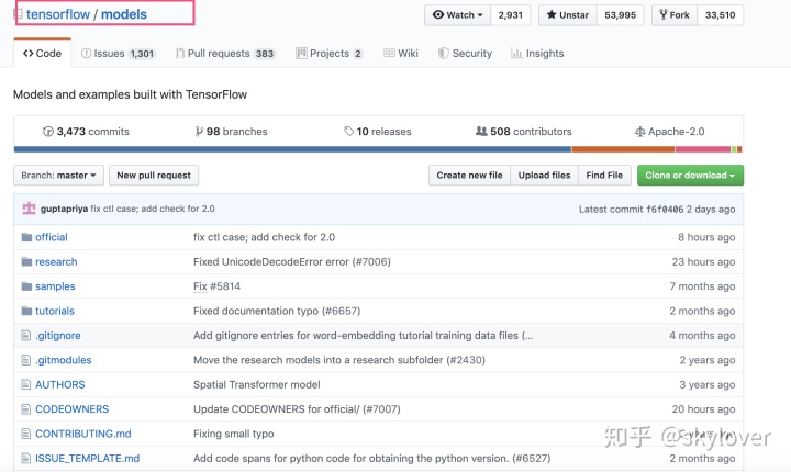
对于计算机视觉:
重点看:compression, im2txt(图像描述),inception (对ImageNet 数据集用Inception V3架构去训练和评估),resnet(残差网络),slim(图像分类)和street(路标识别或验证码识别)
尝试运行上述模型,并对模型进行调试和调参
TensorFlow基本操作
- 卷积
卷积有两种:
“SAME”和“VALID”
对于SAME,输出计算如下:
对于VALID,输出计算如下:
import tensorflow as tf
input = tf.Variable(tf.random_normal([1,4,4,3]))
filter = tf.Variable(tf.random_normal([3,3,3,7]))
result = tf.nn.conv2d(input, filter, strides = [1,3,3,1], padding='SAME')
init = tf.global_variables_initializer()
sess = tf.Session()
sess.run(init)
print(sess.run(result))
print(result.shape)
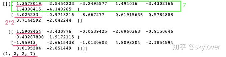
sess.close()输入为443,过滤器为333@7,stride=3.【关于stride 参见[2]】
那么依据响应的规则[3]
n_out = [4 / s] =[4/3]=2*2@7
输出如下:
import tensorflow as tf
input = tf.Variable(tf.random_normal([1,5,5,3]))
filter = tf.Variable(tf.random_normal([3,3,3,7]))

result  = tf.nn.conv2d(input, filter, strides = [1,2,2,1], padding='VALID')
init = tf.global_variables_initializer()

sess = tf.Session()
sess.run(init)

print(sess.run(result))
print(result.shape)

sess.close()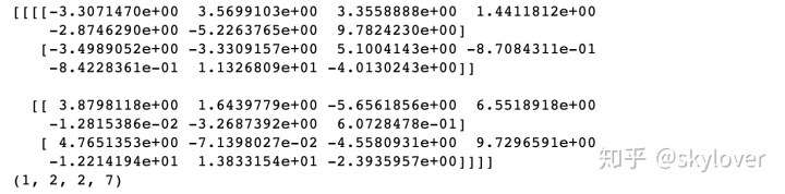
- 池化
tf.nn.max_pool参数含义和用法
- 基本数学操作:
#####################################################
########## Welcome to TensorFlow World ##############
#####################################################
# The tutorials in this section is just a start for math operations.
# The TensorFlow flags are used for having a more user friendly environment.
from __future__ import print_function
import tensorflow as tf
import os
######################################
######### Necessary Flags ############
# ####################################
# The default path for saving event files is the same folder of this python file.
tf.app.flags.DEFINE_string(
'log_dir', os.path.dirname(os.path.abspath(__file__)) + '/logs',
'Directory where event logs are written to.')
# Store all elemnts in FLAG structure!
FLAGS = tf.app.flags.FLAGS
################################################
################# handling errors!##############
################################################
# The user is prompted to input an absolute path.
# os.path.expanduser is leveraged to transform '~' sign to the corresponding path indicator.
# Example: '~/logs' equals to '/home/username/logs'
if not os.path.isabs(os.path.expanduser(FLAGS.log_dir)):
raise ValueError('You must assign absolute path for --log_dir')
# Defining some constant values
a = tf.constant(5.0, name="a")
b = tf.constant(10.0, name="b")
# Some basic operations
x = tf.add(a, b, name="add")
y = tf.div(a, b, name="divide")
# Run the session
with tf.Session() as sess:
writer = tf.summary.FileWriter(os.path.expanduser(FLAGS.log_dir), sess.graph)
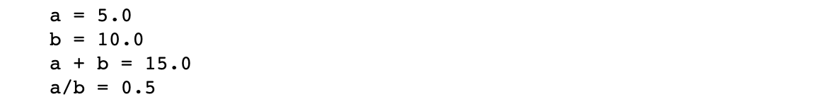
print("a =", sess.run(a))
print("b =", sess.run(b))
print("a + b =", sess.run(x))
print("a/b =", sess.run(y))
# Closing the writer.
writer.close()
sess.close()
除了进行基本的运算外,关于write操作,是为了可视化做准备,会在.py所地方生成 logs ,里面有用于可视化所需记录文件,events.out.tfevents.....
如何可视化?TensorBoard使用【更详细的TB参见[4]】:
在终端输入:tensorboard --logdir /Users/...logs(可以拖进去,如果路径不好找的话)
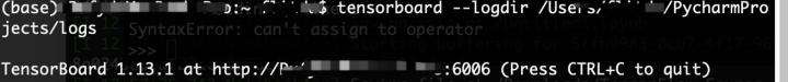
然后会生成一个网址,正常情况下直接粘贴在浏览器即可,但是自己的出现了问题
采用这个替换[5]:
http://localhost:6006
即可得到可视化效果:

===========================================
显示 hello world
#####################################################
########## Welcome to TensorFlow World ##############
#####################################################

# The tutorials in this section is just a start for going into TensorFlow world.
# The TensorFlow flags are used for having a more user friendly environment.

from __future__ import print_function
import tensorflow as tf
import os


################################################
################# handling errors!##############
################################################

# Defining some sentence!
welcome = tf.constant('Welcome to TensorFlow world!')

# Run the session
with tf.Session() as sess:
    print("output: ", sess.run(welcome))

# Closing the writer.

sess.close()
output: b'Welcome to TensorFlow world!'
TensorFlow变量的定义和初始化
Variable() placeholder() constant() 的区别 - 菜鸟后飞
# The tutorials in this section is just a start for math operations.
# The TensorFlow flags are used for having a more user friendly environment.

from __future__ import print_function
import tensorflow as tf
import os
from tensorflow.python.framework import ops


######################################
######### Necessary Flags ############
# ####################################

# The default path for saving event files is the same folder of this python file.
tf.app.flags.DEFINE_string(
    'log_dir', os.path.dirname(os.path.abspath(__file__)) + '/logs',
    'Directory where event logs are written to.')

# Store all elemnts in FLAG structure!
FLAGS = tf.app.flags.FLAGS

################################################
################# handling errors!##############
################################################

# The user is prompted to input an absolute path.
# os.path.expanduser is leveraged to transform '~' sign to the corresponding path indicator.
#       Example: '~/logs' equals to '/home/username/logs'
if not os.path.isabs(os.path.expanduser(FLAGS.log_dir)):
    raise ValueError('You must assign absolute path for --log_dir')


#######################################
######## Defining Variables ###########
#######################################

# Create three variables with some default values.
weights = tf.Variable(tf.random_normal([2, 3], stddev=0.1),
                      name="weights")
biases = tf.Variable(tf.zeros([3]), name="biases")
custom_variable = tf.Variable(tf.zeros([3]), name="custom")

# Get all the variables' tensors and store them in a list.
all_variables_list = ops.get_collection(ops.GraphKeys.GLOBAL_VARIABLES)


############################################
######## Customized initializer ############
############################################

## Initialation of some custom variables.
## In this part we choose some variables and only initialize them rather than initializing all variables.

# "variable_list_custom" is the list of variables that we want to initialize.
variable_list_custom = [weights, custom_variable]

# The initializer
init_custom_op = tf.variables_initializer(var_list=variable_list_custom )


########################################
######## Global initializer ############
########################################

# Method-1
# Add an op to initialize the variables.
init_all_op = tf.global_variables_initializer()

# Method-2
init_all_op = tf.variables_initializer(var_list=all_variables_list)


##########################################################
######## Initialization using other variables ############
##########################################################

# Create another variable with the same value as 'weights'.
WeightsNew = tf.Variable(weights.initialized_value(), name="WeightsNew")

# Now, the variable must be initialized.
init_WeightsNew_op = tf.variables_initializer(var_list=[WeightsNew])

######################################
####### Running the session ##########
######################################
with tf.Session() as sess:
    writer = tf.summary.FileWriter(os.path.expanduser(FLAGS.log_dir), sess.graph)
    # Run the initializer operation.
    sess.run(init_all_op)
    sess.run(init_custom_op)
    sess.run(init_WeightsNew_op)

# Closing the writer.
writer.close()
sess.close()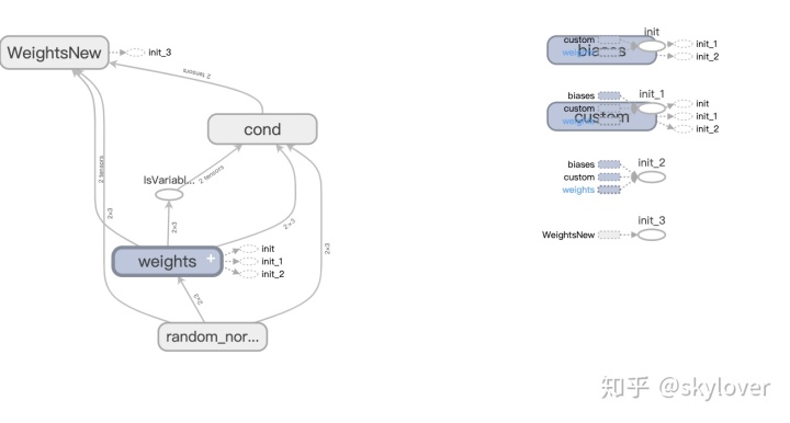
下面例子为简单的线性回归例子,
# coding=utf-8

'''
-------------------------------------------------
Created by Dufy on 2019/4/28
IDE used: PyCharm Community Edition
Description :
1)利用tf进行线性回归的简单练习
2)
-------------------------------------------------
Change Activity:

-------------------------------------------------
'''

import matplotlib.pyplot as plt
import random
import tensorflow as tf
import numpy as np


m = tf.get_variable('m', [], initializer=tf.constant_initializer(0.))
b = tf.get_variable('b', [], initializer=tf.constant_initializer(0.))
init = tf.global_variables_initializer()

input_placeholder = tf.placeholder(tf.float32)
output_placeholder = tf.placeholder(tf.float32)

x = input_placeholder
y = output_placeholder
y_guess = m * x + b

loss = tf.square(y - y_guess)

optimizer = tf.train.GradientDescentOptimizer(1e-3)
train_op = optimizer.minimize(loss)

sess = tf.Session()
sess.run(init)

true_m = random.random()
true_b = random.random()
itera_num = 160
vari_store = np.zeros(shape=(itera_num, 2))
for update_i in range(itera_num):
    input_data = random.random()  # 这里每次提供一个训练数据,而且是随机生成的
    # print(input_data)
    output_data = true_m * input_data + true_b
    _loss, _ = sess.run([loss, train_op], feed_dict={
                        input_placeholder: input_data, output_placeholder: output_data})
    vari_store[update_i][0] = update_i
    vari_store[update_i][1] = _loss
    if update_i % 40 == 0:
        print('更新次数:%.0f, 损失函数:%.9f,运行:%.0f %%' %
              (update_i, _loss, 100 * update_i / itera_num))

print('true parameters: m=%.4f,b=%.4f' % (true_m, true_b))
print('learned parameters: m=%.4f,b=%.4f' % tuple(sess.run([m, b])))
# print(vari_store)
x = vari_store[:, 0]
y = vari_store[:, 1]
# print(x)
plt.plot(x, y, color='blue', linestyle='-', marker='.', label='loss')
# plt.plot(x, y, color='blue', linewidth=1.5, linestyle='-',marker='.',label='loss')
plt.legend(loc='upper right')
plt.show()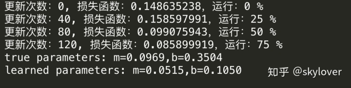
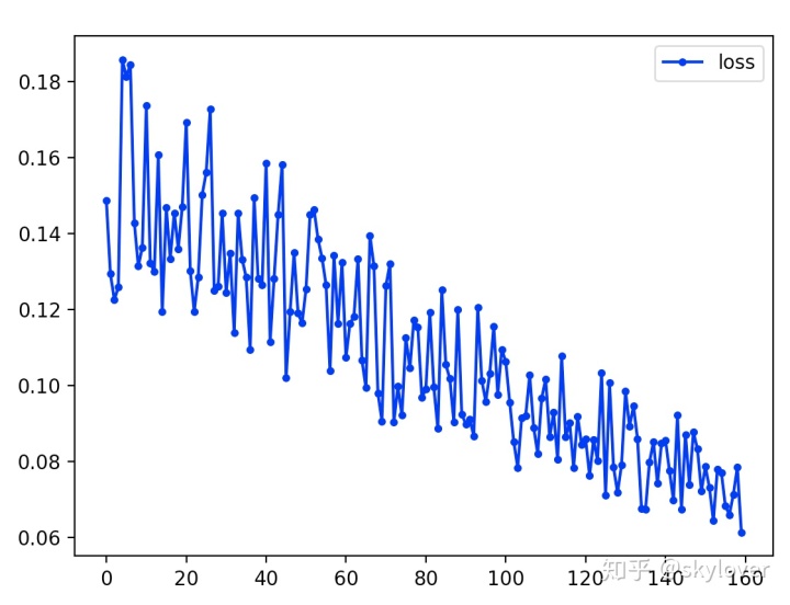
从损失函数图可以看出来,总的趋势是减少的。由于采用的随机梯度下降,所以并不能保证每次都是损失函数减少的。
增加迭代次数,可以得到更好的效果
参考:https://juejin.im/post/5b345a49f265da599c561b25这是我看过解释TensorFlow最透彻的文章!
感知机学习
# coding=utf-8
'''
-------------------------------------------------
Created by Dufy on 2019/4/28
IDE used: PyCharm Community Edition
Description :
1)利用tf进行感知机的学习
2)
-------------------------------------------------
Change Activity:
-------------------------------------------------
'''
import matplotlib.pyplot as plt
import random
import tensorflow as tf
import numpy as np
X = np.array([
[1, 3, 3],
[1, 4, 3],
[1, 1, 1],
[1, 4, 1],
[1, 0, -2]
])
# 为什么样本坐标是 [3,3][4,3][1,1] 而这里多了个1 变成了
# [1, 3, 3],
# [1, 4, 3],
# [1, 1, 1]
# 因为 函数方程有一个常数项 比如 5 + x + 2y = 0 这里面的5 即是常数项。
# 如果矩阵没有第一位为1 则这个常数项无法体现
# 期望输出值
Y = np.array([1, 1, -1, 1, -1])
# 权重初始化 一行三列矩阵,取值范围 -1到1
W = (np.random.random(3) - 0.5) * 2
# 学习率
lr = 0.11
# 记录 循环点带次数
n = 0
# 输出值
O = 0
def update():
global X, Y, W, lr, n
n += 1
# 矩阵乘法 也即是 (3行3列)矩阵X 乘以 1列矩阵W.T
# (一行矩阵W, W.T 是将矩阵偏转成 1列)
# 其中 np.dat() 是矩阵相乘, 返回一个矩阵结果 在这里返回的是一个 3行1列
# np.sign() 返回数组中各元素的正负符号,用1和-1表示 数组元素分类
O = np.sign(np.dot(X, W.T))
''' 获取改变权值 这一块比较难懂。
因为我们的目的是在坐标上找到一根直线 来区分正样本和负样本
也即是 输入矩阵X
X = np.array([
[1, 3, 3],
[1, 4, 3],
[1, 1, 1]
])
用权重矩阵W和X的每行相乘。 这里W矩阵为 [w0,w1,w2]
例如X的第一行和W相乘 1*w0 + 3*w1 + 3*w2
最后 X*W.T会得到一个3行1列矩阵, 我们用np.sign() 返回数组中各元素的正负符号,
用1和-1表示 数组元素分类
最后会得到矩阵 O。 当矩阵O和期望输出 Y = np.array([1, 1, -1]) 相等时 我们的权重则计算完成
当我们获取到这个权重后, 我们就可以拿这个权重 去生成一个方程 w0 + x*w1 + y*w2=0
这个方程 输入我们的正样本 得出正值 输入负样本得出负值
这个方程 也即是 y = (-x*w1/w2) + (-w0/w2)
也即是 斜率为 -w1/w2 截距为 -w0/w2
'''
W_C = lr * (Y - O.T).dot(X) / int(X.shape[0])
W = W + W_C
for _ in range(100):
update()
O = np.sign(np.dot(X, W.T))
if (O == Y.T).all(): # 如果实际输出等于期望输出 循环结束
break
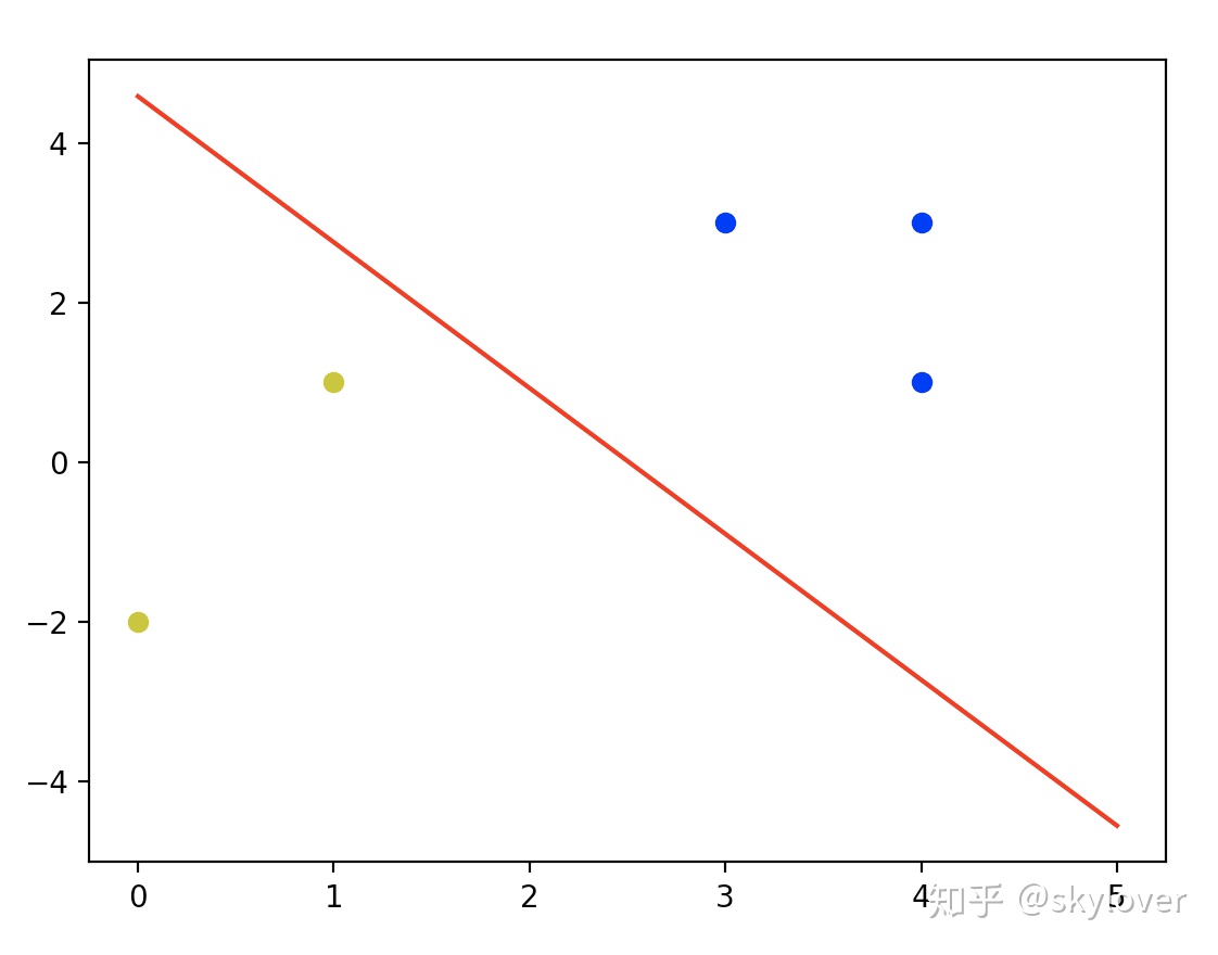
# 正样本
x1 = [3, 4, 4]
y1 = [3, 3, 1]
# 负样本
x2 = [1, 0]
y2 = [1, -2]
# k是斜率 d是截距 获取方式 在权重那块写了
k = -W[1] / W[2]
d = -W[0] / W[2]
'''生成图片显示出效果'''
xdata = np.linspace(0, 5)
plt.figure()
plt.plot(xdata, xdata * k + d, 'r')
plt.plot(x1, y1, 'bo')
plt.plot(x2, y2, 'yo')
plt.show()
# 反向传播
#----------------------------------
#
# 以下Python函数主要是展示回归和分类模型的反向传播

import matplotlib.pyplot as plt
import numpy as np
import tensorflow as tf
from tensorflow.python.framework import ops
ops.reset_default_graph()

# 创建计算图会话
sess = tf.Session()

# 回归算法的例子:
# We will create sample data as follows:
# x-data: 100 random samples from a normal ~ N(1, 0.1)
# target: 100 values of the value 10.
# We will fit the model:
# x-data * A = target
# Theoretically, A = 10.

# 生成数据,创建占位符和变量A
x_vals = np.random.normal(1, 0.1, 100)
y_vals = np.repeat(10., 100)
x_data = tf.placeholder(shape=[1], dtype=tf.float32)
y_target = tf.placeholder(shape=[1], dtype=tf.float32)

# Create variable (one model parameter = A)
A = tf.Variable(tf.random_normal(shape=[1]))

# 增加乘法操作
my_output = tf.multiply(x_data, A)

# 增加L2正则损失函数
loss = tf.square(my_output - y_target)

# 在运行优化器之前,需要初始化变量
init = tf.global_variables_initializer()
sess.run(init)

# 声明变量的优化器
my_opt = tf.train.GradientDescentOptimizer(0.02)
train_step = my_opt.minimize(loss)

# 训练算法
for i in range(100):
    rand_index = np.random.choice(100)
    rand_x = [x_vals[rand_index]]
    rand_y = [y_vals[rand_index]]
    sess.run(train_step, feed_dict={x_data: rand_x, y_target: rand_y})
    if (i+1)%25==0:
        print('Step #' + str(i+1) + ' A = ' + str(sess.run(A)))
        print('Loss = ' + str(sess.run(loss, feed_dict={x_data: rand_x, y_target: rand_y})))
============================================================
# 分类算法例子
# We will create sample data as follows:
# x-data: sample 50 random values from a normal = N(-1, 1)
#         + sample 50 random values from a normal = N(1, 1)
# target: 50 values of 0 + 50 values of 1.
#         These are essentially 100 values of the corresponding output index
# We will fit the binary classification model:
# If sigmoid(x+A) < 0.5 -> 0 else 1
# Theoretically, A should be -(mean1 + mean2)/2

# 重置计算图
ops.reset_default_graph()

# Create graph
sess = tf.Session()

# 生成数据
x_vals = np.concatenate((np.random.normal(-1, 1, 50), np.random.normal(3, 1, 50)))
y_vals = np.concatenate((np.repeat(0., 50), np.repeat(1., 50)))
x_data = tf.placeholder(shape=[1], dtype=tf.float32)
y_target = tf.placeholder(shape=[1], dtype=tf.float32)

# 偏差变量A (one model parameter = A)
A = tf.Variable(tf.random_normal(mean=10, shape=[1]))

# 增加转换操作
# Want to create the operstion sigmoid(x + A)
# Note, the sigmoid() part is in the loss function
my_output = tf.add(x_data, A)

# 由于指定的损失函数期望批量数据增加一个批量数的维度
# 这里使用expand_dims()函数增加维度
my_output_expanded = tf.expand_dims(my_output, 0)
y_target_expanded = tf.expand_dims(y_target, 0)

# 初始化变量A
init = tf.global_variables_initializer()
sess.run(init)

# 声明损失函数 交叉熵(cross entropy)
xentropy = tf.nn.sigmoid_cross_entropy_with_logits(logits=my_output_expanded, labels=y_target_expanded)

# 增加一个优化器函数 让TensorFlow知道如何更新和偏差变量
my_opt = tf.train.GradientDescentOptimizer(0.05)
train_step = my_opt.minimize(xentropy)

# 迭代
for i in range(1400):
    rand_index = np.random.choice(100)
    rand_x = [x_vals[rand_index]]
    rand_y = [y_vals[rand_index]]

    sess.run(train_step, feed_dict={x_data: rand_x, y_target: rand_y})
    if (i+1)%200==0:
        print('Step #' + str(i+1) + ' A = ' + str(sess.run(A)))
        print('Loss = ' + str(sess.run(xentropy, feed_dict={x_data: rand_x, y_target: rand_y})))

# 评估预测
predictions = []
for i in range(len(x_vals)):
    x_val = [x_vals[i]]
    prediction = sess.run(tf.round(tf.sigmoid(my_output)), feed_dict={x_data: x_val})
    predictions.append(prediction[0])

accuracy = sum(x==y for x,y in zip(predictions, y_vals))/100.
print('最终精确度 = ' + str(np.round(accuracy, 2)))
参考
- ^如何理解深度学习源码里经常出现的logits? https://www.zhihu.com/question/60751553
- ^ TensorFlow strides 参数讨论 https://blog.csdn.net/lanchunhui/article/details/61615714
- ^原 TensorFlow中padding卷积的两种方式“SAME”和“VALID” https://blog.csdn.net/syyyy712/article/details/80272071
- ^TensorFlow——可视化工具TensorBoard的使用 https://blog.csdn.net/asialee_bird/article/details/80202351
- ^执行 tensorboard --logdir logs之后遇到的浏览器中输入http://localhost:6006 网址打不开的问题 https://blog.csdn.net/sinat_28442665/article/details/81076600


 4445
4445


 被折叠的 条评论
为什么被折叠?
被折叠的 条评论
为什么被折叠?
 到【灌水乐园】发言


