matplotlib 显示批量图片_使用Matplotlib对数据进行高级可视化(基本图，3D图和小部件)...

作者 | Veekesh Dhununjoy

来源 | Medium

编辑 | 代码医生团队

一张图片胜过千言万语，良好的可视化价值数百万。

可视化在当今世界许多领域的结果传播中发挥着重要作用。如果没有适当的可视化，很难揭示结果，理解变量之间的复杂关系并描述数据的趋势。

本文将首先使用Matplotlib绘制基本图，然后深入研究一些非常有用的高级可视化技术，如“mplot3d Toolkit”(生成3D图)和小部件。

在温哥华房产税报表数据集已经被用于探索不同类型的地块在Matplotlib库。该数据集包含有关BC评估(BCA)和城市来源的属性的信息，包括物业ID，建成年份，区域类别，当前土地价值等。

文章底部提到了代码的链接。

Matplotlib基本图

给定示例中经常使用的命令：

plt.figure()：创建一个新的数字

https://matplotlib.org/api/_as_gen/matplotlib.pyplot.figure.html

plt.plot()：绘制y与x作为行和/或标记

https://matplotlib.org/api/_as_gen/matplotlib.pyplot.plot.html

plt.xlabel()：设置x轴的标签

https://matplotlib.org/api/_as_gen/matplotlib.pyplot.xlabel.html

plt.ylabel()：设置标签对于y轴

https://matplotlib.org/api/_as_gen/matplotlib.pyplot.ylabel.html

plt.title()：设置轴的标题

https://matplotlib.org/api/_as_gen/matplotlib.pyplot.title.html

plt.grid()：配置网格线

https://matplotlib.org/api/_as_gen/matplotlib.pyplot.grid.html

plt.legend()：在轴上放置图例

https://matplotlib.org/api/_as_gen/matplotlib.pyplot.legend.html

plt.savefig()：保存当前图形在磁盘上

https://matplotlib.org/api/_as_gen/matplotlib.pyplot.savefig.html

plt.show()：显示图形

https://matplotlib.org/api/_as_gen/matplotlib.pyplot.show.html

plt.clf()：清除当前图形(用于在同一代码中绘制多个图形)

https://matplotlib.org/api/_as_gen/matplotlib.pyplot.clf.html

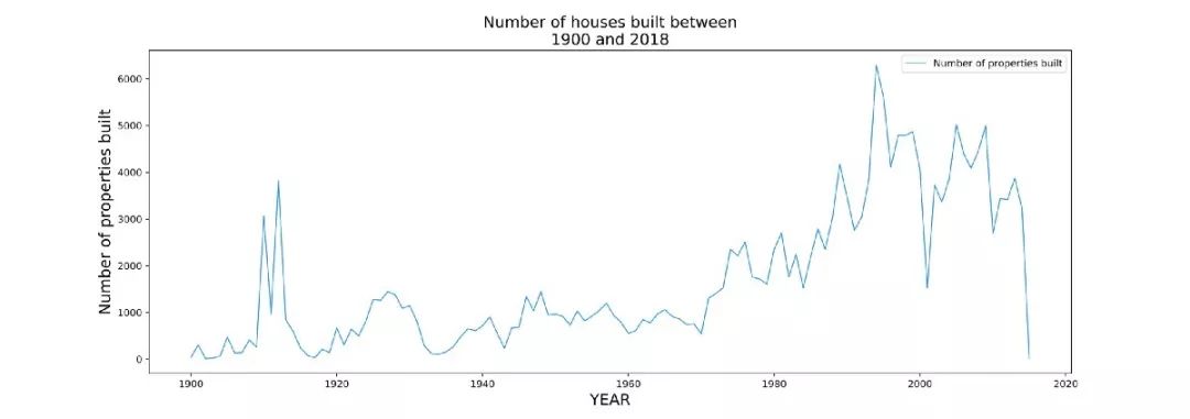
1.线图

线图是一个基本图表，它将信息显示为一系列称为由直线段连接的标记的数据点。

# Line plot.# Importing matplotlib to plot the graphs.import matplotlib.pyplot as plt# Importing pandas for using pandas dataframes.import pandas as pd# Reading the input file.
df = pd.read_csv("property_tax_report_2018.csv")# Removing the null values in PROPERTY_POSTAL_CODE.
df = df[(df['PROPERTY_POSTAL_CODE'].notnull())]# Grouping by YEAR_BUILT and aggregating based on PID to count the number of properties for each year.
df = df[['PID', 'YEAR_BUILT']].groupby('YEAR_BUILT', as_index = False).count().astype('int').rename(columns = {'PID':'No_of_properties_built'})# Filtering YEAR_BUILT and keeping only the values between 1900 to 2018.
df = df[(df['YEAR_BUILT'] >= 1900) & (df['YEAR_BUILT'] <= 2018)]# X-axis: YEAR_BUILT
x = df['YEAR_BUILT']# Y-axis: Number of properties built.
y = df['No_of_properties_built']# Change the size of the figure (in inches).
plt.figure(figsize=(17,6))# Plotting the graph using x and y with 'dodgerblue' color.# Different labels can be given to different lines in the same plot.# Linewidth determines the width of the line.
plt.plot(x, y, 'dodgerblue', label = 'Number of properties built', linewidth = 1)# plt.plot(x2, y2, 'red', label = 'Line 2', linewidth = 2)# X-axis label.
plt.xlabel('YEAR', fontsize = 16)# Y-axis label.
plt.ylabel('Number of properties built', fontsize = 16)# Title of the plot.
plt.title('Number of houses built between\n1900 and 2018', fontsize = 16)# Grid# plt.grid(True)
plt.grid(False)# Legend for the plot.
plt.legend()# Saving the figure on disk. 'dpi' and 'quality' can be adjusted according to the required image quality.
plt.savefig('Line_plot.jpeg', dpi = 400, quality = 100)# Displays the plot.
plt.show()# Clears the current figure contents.
plt.clf()

上面的代码段可用于创建折线图。在这里Pandas Dataframe已被用于执行基本数据操作。在读取和处理输入数据集之后，使用plt.plot()绘制x轴上的Year和在y轴上构建的属性数的折线图。

2.Bar Plot

条形图显示具有与其表示的值成比例的矩形高度或长度条的分类数据。

# Bar plot.# Importing matplotlib to plot the graphs.import matplotlib.pyplot as plt# Importing pandas for using pandas dataframes.import pandas as pd# Reading the input file.
df = pd.read_csv("property_tax_report_2018.csv")# Removing the null values in PROPERTY_POSTAL_CODE.
df = df[(df['PROPERTY_POSTAL_CODE'].notnull())]# Grouping by YEAR_BUILT and aggregating based on PID to count the number of properties for each year.
df = df[['PID', 'YEAR_BUILT']].groupby('YEAR_BUILT', as_index = False).count().astype('int').rename(columns = {'PID':'No_of_properties_built'})# Filtering YEAR_BUILT and keeping only the values between 1900 to 2018.
df = df[(df['YEAR_BUILT'] >= 1900) & (df['YEAR_BUILT'] <= 2018)]# X-axis: YEAR_BUILT
x = df['YEAR_BUILT']# Y-axis: Number of properties built.
y = df['No_of_properties_built']# Change the size of the figure (in inches).
plt.figure(figsize=(17,6))# Plotting the graph using x and y with 'dodgerblue' color.# Different labels can be given to different bar plots in the same plot.# Linewidth determines the width of the line.
plt.bar(x, y, label = 'Number of properties built', color = 'dodgerblue',  width = 1,, alpha = 0.7)# plt.bar(x2, y2, label = 'Bar 2', color = 'red',  width = 1)# X-axis label.
plt.xlabel('YEAR', fontsize = 16)# Y-axis label.
plt.ylabel('Number of properties built', fontsize = 16)# Title of the plot.
plt.title('Number of houses built between\n1900 and 2018', fontsize = 16)# Grid# plt.grid(True)
plt.grid(axis='y')# Legend for the plot.
plt.legend()# Saving the figure on disk. 'dpi' and 'quality' can be adjusted according to the required image quality.
plt.savefig('Bar_plot.jpeg', dpi = 400, quality = 100)# Displays the plot.
plt.show()# Clears the current figure contents.
plt.clf()

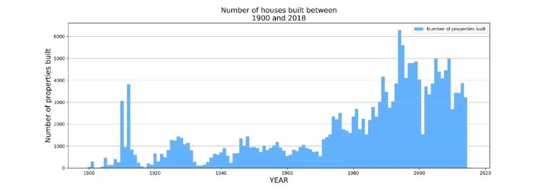
上面的代码段可用于创建条形图。

3.直方图

直方图是数值数据分布的精确表示。它是连续变量的概率分布的估计。

# Histogram# Importing matplotlib to plot the graphs.import matplotlib.pyplot as plt# Importing pandas for using pandas dataframes.import pandas as pd# Reading the input file.
df = pd.read_csv("property_tax_report_2018.csv")# Removing the null values in PROPERTY_POSTAL_CODE.
df = df[(df['PROPERTY_POSTAL_CODE'].notnull())]# Grouping by YEAR_BUILT and aggregating based on PID to count the number of properties for each year.
df = df[['PID', 'YEAR_BUILT']].groupby('YEAR_BUILT', as_index = False).count().astype('int').rename(columns = {'PID':'No_of_properties_built'})# Filtering YEAR_BUILT and keeping only the values between 1900 to 2018.
df = df[(df['YEAR_BUILT'] >= 1900) & (df['YEAR_BUILT'] <= 2018)]# Change the size of the figure (in inches).
plt.figure(figsize=(17,6))# X-axis: Number of properties built from 1900 to 2018.# Y-axis: Frequency.
plt.hist(df['No_of_properties_built'],
         bins = 50,
         histtype='bar',
         rwidth = 1.0,
         color = 'dodgerblue',
         alpha = 0.8
       )# X-axis label.
plt.xlabel('Number of properties built from 1900 to 2018', fontsize = 16)# Y-axis label.
plt.ylabel('Frequency', fontsize = 16)# Title of the plot.
plt.title('Distribution of the number of properties built between 1900 and 2018.', fontsize = 16)# Grid# plt.grid(True)
plt.grid(axis='y')# Saving the figure on disk. 'dpi' and 'quality' can be adjusted according to the required image quality.
plt.savefig('Histogram.jpeg', dpi = 400, quality = 100)# Displays the plot.
plt.show()# Clears the current figure contents.
plt.clf()

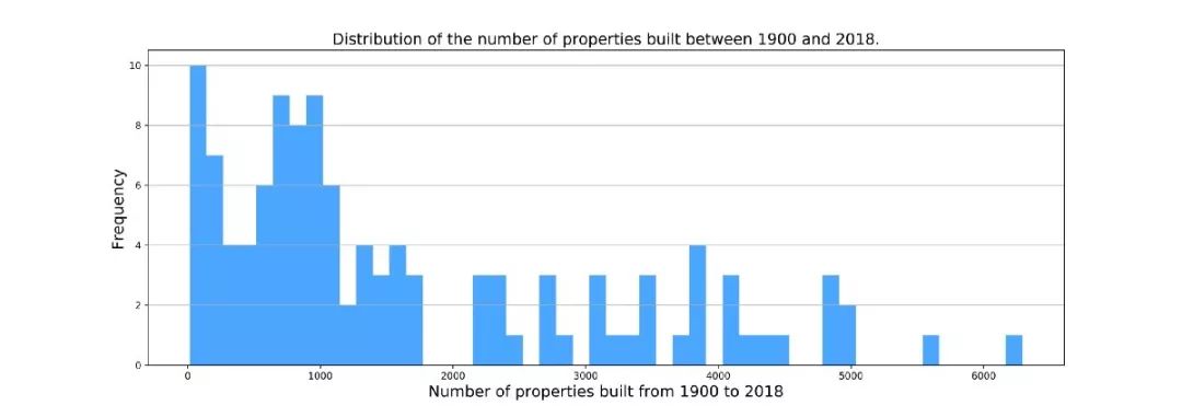
上面的代码段可用于创建直方图。

4.饼图

饼图是圆形统计图形，其被分成切片以示出数字比例。在饼图中每个切片的弧长与其表示的数量成比例。

# Pie-chart.# Importing matplotlib to plot the graphs.import matplotlib.pyplot as plt# Importing pandas for using pandas dataframes.import pandas as pd# Reading the input file.
df = pd.read_csv("property_tax_report_2018.csv")# Filtering out the null values in ZONE_CATEGORY
df = df[df['ZONE_CATEGORY'].notnull()]# Grouping by ZONE_CATEGORY and aggregating based on PID to count the number of properties for a particular zone.
df_zone_properties = df.groupby('ZONE_CATEGORY', as_index=False)['PID'].count().rename(columns = {'PID':'No_of_properties'})# Counting the total number of properties.
total_properties = df_zone_properties['No_of_properties'].sum()# Calculating the percentage share of each ZONE for the number of properties in the total number of properties.
df_zone_properties['percentage_of_properties'] = ((df_zone_properties['No_of_properties'] / total_properties) * 100)# Finding the ZONES with the top-5 percentage share in the total number of properties.
df_top_10_zone_percentage = df_zone_properties.nlargest(columns='percentage_of_properties', n = 5)# Change the size of the figure (in inches).
plt.figure(figsize=(8,6))# Slices: percentage_of_properties.
slices = df_top_10_zone_percentage['percentage_of_properties']# Categories: ZONE_CATEGORY.
categories = df_top_10_zone_percentage['ZONE_CATEGORY']# For different colors: https://matplotlib.org/examples/color/named_colors.html
cols = ['purple', 'red', 'green', 'orange', 'dodgerblue']# Plotting the pie-chart.
plt.pie(slices,
        labels = categories,
        colors=cols,
        startangle = 90,#         shadow = True,# To drag the slices away from the centre of the plot.
        explode = (0.040,0,0,0,0),# To display the percent value using Python string formatting.
        autopct = '%1.1f%%'
       )# Title of the plot.
plt.title('Top-5 zone categories with the highest percentage\nshare in the total number of properties.', fontsize = 12)# Saving the figure on disk. 'dpi' and 'quality' can be adjusted according to the required image quality.
plt.savefig('Pie_chart.jpeg', dpi = 400, quality = 100)# Displays the plot.
plt.show()# Clears the current figure contents.
plt.clf()

上面的代码段可用于创建饼图。

5.散点图

# Scatter plot.# Importing matplotlib to plot the graphs.import matplotlib.pyplot as plt# Importing pandas for using pandas dataframes.import pandas as pd# Reading the input file.
df = pd.read_csv("property_tax_report_2018.csv")# Removing the null values in PROPERTY_POSTAL_CODE.
df = df[(df['PROPERTY_POSTAL_CODE'].notnull())]# Grouping by YEAR_BUILT and aggregating based on PID to count the number of properties for each year.
df = df[['PID', 'YEAR_BUILT']].groupby('YEAR_BUILT', as_index = False).count().astype('int').rename(columns = {'PID':'No_of_properties_built'})# Filtering YEAR_BUILT and keeping only the values between 1900 to 2018.
df = df[(df['YEAR_BUILT'] >= 1900) & (df['YEAR_BUILT'] <= 2018)]# X-axis: YEAR_BUILT
x = df['YEAR_BUILT']# Y-axis: Number of properties built.
y = df['No_of_properties_built']# Change the size of the figure (in inches).
plt.figure(figsize=(17,6))# Plotting the scatter plot.# For different types of markers: https://matplotlib.org/api/markers_api.html#module-matplotlib.markers
plt.scatter(x, y, label = 'Number of properties built',s = 200, color = 'red',
            alpha = 0.8, marker = '.', edgecolors='black')# X-axis label.
plt.xlabel('YEAR', fontsize = 16)# Y-axis label.
plt.ylabel('Number of properties built', fontsize = 16)# Title of the plot.
plt.title('Number of houses built between\n1900 and 2018', fontsize = 16)# Grid# plt.grid(True)
plt.grid(axis='y')# Legend for the plot.
plt.legend()# Saving the figure on disk. 'dpi' and 'quality' can be adjusted according to the required image quality.
plt.savefig('Scatter_plot.jpeg', dpi = 400, quality = 100)# Displays the plot.
plt.show()# Clears the current figure contents.
plt.clf()

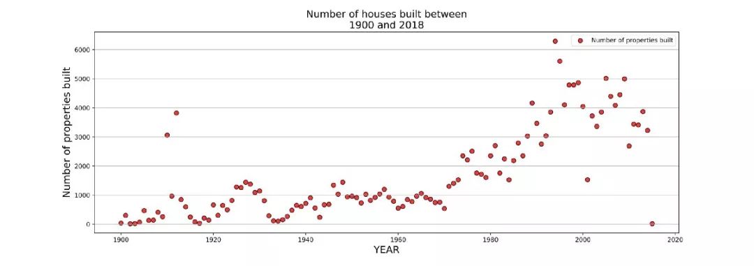
上面的代码段可用于创建散点图。

6.使用图像

下载Lenna测试图像。(来源：维基百科)

https://upload.wikimedia.org/wikipedia/en/7/7d/Lenna_%28test_image%29.png?

# Reading, displaying and saving an image.# Importing matplotlib pyplot and image.import matplotlib.pyplot as pltimport matplotlib.image as mpimg# Reading the image from the disk.
image = mpimg.imread('Lenna_test_image.png')# Displaying the image.
plt.imshow(image)# Saving the image on the disk.
plt.imsave('save_Lenna.png', image, format = 'png')

使用Matplotlib的3D绘图

3D图在三维或多维可视化复杂数据中起着重要作用。

1.3D散点图

'''
==============
3D scatterplot
==============
Demonstration of a basic scatterplot in 3D.
'''# Import librariesfrom mpl_toolkits.mplot3d import Axes3Dimport matplotlib.pyplot as pltfrom matplotlib.lines import Line2Dimport numpy as npimport pandas as pd# Create figure object
fig = plt.figure()# Get the current axes, creating one if necessary.
ax = fig.gca(projection='3d')# Get the Property Tax Report dataset# Dataset link: https://data.vancouver.ca/datacatalogue/propertyTax.htm
data = pd.read_csv('property_tax_report_2018.csv')# Extract the columns and do some transformations
yearWiseAgg = data[['PID','CURRENT_LAND_VALUE']].groupby(data['YEAR_BUILT']).agg({'PID':'count','CURRENT_LAND_VALUE':'sum'})
yearWiseAgg = yearWiseAgg.reset_index().dropna()# Define colors as red, green, blue
colors = ['r', 'g', 'b']# Get only records which have more than 2000 properties built per year
morethan2k = yearWiseAgg.query('PID>2000')# Get shape of dataframe
dflen = morethan2k.shape[0]# Fetch land values from dataframe
lanvalues = (morethan2k['CURRENT_LAND_VALUE']/2e6).tolist()# Create a list of colors for each point corresponding to x and y
c_list = []for i,value in enumerate(lanvalues):if value>0 and value<1900:
        c_list.append(colors[0])elif value>=1900 and value<2900:
        c_list.append(colors[1])else:
        c_list.append(colors[2])# By using zdir='y', the y value of these points is fixed to the zs value 0# and the (x,y) points are plotted on the x and z axes.
ax.scatter(morethan2k['PID'], morethan2k['YEAR_BUILT'], morethan2k['CURRENT_LAND_VALUE']/2e6,c=c_list)# Set labels according to axis
plt.xlabel('Number of Properties')
plt.ylabel('Year Built')
ax.set_zlabel('Current land value (million)')# Create customized legends
legend_elements = [Line2D([0], [0], marker='o', color='w', label='No. of Properties with sum of land value price less than 1.9 millions',markerfacecolor='r', markersize=10),
                  Line2D([0], [0], marker='o', color='w', label='Number of properties with their land value price less than 2.9 millions',markerfacecolor='g', markersize=10),
                   Line2D([0], [0], marker='o', color='w', label='Number of properties with their land values greater than 2.9 millions',markerfacecolor='b', markersize=10)
                  ]# Make legend
ax.legend(handles=legend_elements, loc='best')
plt.show()

3D散点图用于绘制三个轴上的数据点，以试图显示三个变量之间的关系。数据表中的每一行都由一个标记表示，该标记的位置取决于在X，Y和Z轴上设置的列中的值。

2.3D线图

'''
==============
3D lineplot
==============
Demonstration of a basic lineplot in 3D.
'''# Import librariesimport matplotlib as mplfrom mpl_toolkits.mplot3d import Axes3Dimport numpy as npimport matplotlib.pyplot as plt# Set the legend font size to 10
mpl.rcParams['legend.fontsize'] = 10# Create figure object
fig = plt.figure()# Get the current axes, creating one if necessary.
ax = fig.gca(projection='3d')# Create data point to plot
theta = np.linspace(-4 * np.pi, 4 * np.pi, 100)
z = np.linspace(-2, 2, 100)
r = z**2 + 1
x = r * np.sin(theta)
y = r * np.cos(theta)# Plot line graph
ax.plot(x, y, z, label='Parametric curve')# Set default legend
ax.legend()
plt.show()

当有一个不断增加或减少的变量时，可以使用3D线图。该变量可以放置在Z轴上，而其他两个变量的变化可以在X轴和Y轴上观察到Z轴。例如使用时间序列数据(例如行星运动)，则可以将时间放在Z轴上，并且可以从可视化中观察其他两个变量的变化。

3.3D图作为子图

'''
====================
3D plots as subplots
====================
Demonstrate including 3D plots as subplots.
'''import matplotlib.pyplot as pltfrom mpl_toolkits.mplot3d.axes3d import Axes3D, get_test_datafrom matplotlib import cmimport numpy as np# set up a figure twice as wide as it is tall
fig = plt.figure(figsize=plt.figaspect(0.5))#===============#  First subplot#===============# set up the axes for the first plot
ax = fig.add_subplot(1, 2, 1, projection='3d')# plot a 3D surface like in the example mplot3d/surface3d_demo# Get equally spaced numbers with interval of 0.25 from -5 to 5
X = np.arange(-5, 5, 0.25)
Y = np.arange(-5, 5, 0.25)# Convert it into meshgrid for plotting purpose using x and y
X, Y = np.meshgrid(X, Y)
R = np.sqrt(X**2 + Y**2)
Z = np.sin(R)
surf = ax.plot_surface(X, Y, Z, rstride=1, cstride=1, cmap=cm.coolwarm,
                       linewidth=0, antialiased=False)
ax.set_zlim(-1.01, 1.01)
fig.colorbar(surf, shrink=0.5, aspect=10)#===============# Second subplot#===============# set up the axes for the second plot
ax = fig.add_subplot(1, 2, 2, projection='3d')# plot a 3D wireframe like in the example mplot3d/wire3d_demo# Return a tuple X, Y, Z with a test data set
X, Y, Z = get_test_data(0.05)
ax.plot_wireframe(X, Y, Z, rstride=10, cstride=10)
plt.show()

上面的代码片段可用于创建多个3D绘图作为同一图中的子图。两个图都可以独立分析。

4.轮廓图

'''
==============
Contour Plots
==============
Plot a contour plot that shows intensity
'''# Import librariesfrom mpl_toolkits.mplot3d import axes3dimport matplotlib.pyplot as pltfrom matplotlib import cm# Create figure object
fig = plt.figure()# Get the current axes, creating one if necessary.
ax = fig.gca(projection='3d')# Get test data
X, Y, Z = axes3d.get_test_data(0.05)# Plot contour curves
cset = ax.contour(X, Y, Z, cmap=cm.coolwarm)# Set labels
ax.clabel(cset, fontsize=9, inline=1)
plt.show()

上面的代码片段可用于创建等高线图。轮廓图可用于表示2D格式的3D表面。给定Z轴的值，绘制线以连接发生特定z值的(x，y)坐标。轮廓图通常用于连续变量而不是分类数据。

5.具有强度的轮廓图

'''
==============
Contour Plots
==============
Plot a contour plot that shows intensity
'''# Import librariesfrom mpl_toolkits.mplot3d import axes3dimport matplotlib.pyplot as pltfrom matplotlib import cm# Create figure object
fig = plt.figure()# Get the current axes, creating one if necessary.
ax = fig.gca(projection='3d')# Get test data
X, Y, Z = axes3d.get_test_data(0.05)# Plot contour curves
cset = ax.contourf(X, Y, Z, cmap=cm.coolwarm)# Set labels
ax.clabel(cset, fontsize=9, inline=1)
plt.show()

上面的代码片段可用于创建填充的等高线图。

6.表面图

"""
========================
Create 3d surface plots
========================
Plot a contoured surface plot
"""# Import librariesfrom mpl_toolkits.mplot3d import Axes3Dimport matplotlib.pyplot as pltfrom matplotlib import cmfrom matplotlib.ticker import LinearLocator, FormatStrFormatterimport numpy as np# Create figures object
fig = plt.figure()# Get the current axes, creating one if necessary.
ax = fig.gca(projection='3d')# Make data.
X = np.arange(-5, 5, 0.25)
Y = np.arange(-5, 5, 0.25)
X, Y = np.meshgrid(X, Y)
R = np.sqrt(X**2 + Y**2)
Z = np.sin(R)# Plot the surface.
surf = ax.plot_surface(X, Y, Z, cmap=cm.coolwarm,
                       linewidth=0, antialiased=False)# Customize the z axis.
ax.set_zlim(-1.01, 1.01)
ax.zaxis.set_major_locator(LinearLocator(10))
ax.zaxis.set_major_formatter(FormatStrFormatter('%.02f'))# Add a color bar which maps values to colors.
fig.colorbar(surf, shrink=0.5, aspect=5)
plt.show()

上面的代码段可用于创建用于绘制3D数据的Surface图。它们显示指定的因变量(Y)和两个独立变量(X和Z)之间的函数关系，而不是显示各个数据点。上述图的实际应用是可视化梯度下降算法如何汇合。

7.三角形曲面图

'''
======================
Triangular 3D surfaces
======================
Plot a 3D surface with a triangular mesh.
'''# Import librariesfrom mpl_toolkits.mplot3d import Axes3D  import matplotlib.pyplot as pltimport numpy as np# Create figures object
fig = plt.figure()# Get the current axes, creating one if necessary.
ax = fig.gca(projection='3d')# Set parameters
n_radii = 8
n_angles = 36# Make radii and angles spaces (radius r=0 omitted to eliminate duplication).
radii = np.linspace(0.125, 1.0, n_radii)
angles = np.linspace(0, 2*np.pi, n_angles, endpoint=False)[..., np.newaxis]# Convert polar (radii, angles) coords to cartesian (x, y) coords.# (0, 0) is manually added at this stage,  so there will be no duplicate# points in the (x, y) plane.
x = np.append(0, (radii*np.cos(angles)).flatten())
y = np.append(0, (radii*np.sin(angles)).flatten())# Compute z to make the pringle surface.
z = np.sin(-x*y)# Plot triangular meshed surface plot
ax.plot_trisurf(x, y, z, linewidth=0.2, antialiased=True)
plt.show()

上面的代码片段可用于创建三角曲面图。

8.多边形图

'''
==============
Polygon Plots
==============
Plot a polygon plot
'''# Import librariesfrom mpl_toolkits.mplot3d import Axes3D  from matplotlib.collections import PolyCollectionimport matplotlib.pyplot as pltfrom matplotlib import colors as mcolorsimport numpy as np# Fixing random state for reproducibility
np.random.seed(19680801)def cc(arg):'''
    Shorthand to convert 'named' colors to rgba format at 60% opacity.
    '''return mcolors.to_rgba(arg, alpha=0.6)def polygon_under_graph(xlist, ylist):'''
    Construct the vertex list which defines the polygon filling the space under
    the (xlist, ylist) line graph.  Assumes the xs are in ascending order.
    '''return [(xlist[0], 0.), *zip(xlist, ylist), (xlist[-1], 0.)]# Create figure object
fig = plt.figure()# Get the current axes, creating one if necessary.
ax = fig.gca(projection='3d')# Make verts a list, verts[i] will be a list of (x,y) pairs defining polygon i
verts = []# Set up the x sequence
xs = np.linspace(0., 10., 26)# The ith polygon will appear on the plane y = zs[i]
zs = range(4)for i in zs:
    ys = np.random.rand(len(xs))
    verts.append(polygon_under_graph(xs, ys))
poly = PolyCollection(verts, facecolors=[cc('r'), cc('g'), cc('b'), cc('y')])
ax.add_collection3d(poly, zs=zs, zdir='y')# Set labels
ax.set_xlabel('X')
ax.set_ylabel('Y')
ax.set_zlabel('Z')
ax.set_xlim(0, 10)
ax.set_ylim(-1, 4)
ax.set_zlim(0, 1)
plt.show()

上面的代码片段可用于创建多边形图。

9.3D中的文本注释

'''
======================
Text annotations in 3D
======================
Demonstrates the placement of text annotations on a 3D plot.
Functionality shown:
- Using the text function with three types of 'zdir' values: None,
  an axis name (ex. 'x'), or a direction tuple (ex. (1, 1, 0)).
- Using the text function with the color keyword.
- Using the text2D function to place text on a fixed position on the ax object.
'''# Import librariesfrom mpl_toolkits.mplot3d import Axes3Dimport matplotlib.pyplot as plt# Create figure object
fig = plt.figure()# Get the current axes, creating one if necessary.
ax = fig.gca(projection='3d')# Demo 1: zdir
zdirs = (None, 'x', 'y', 'z', (1, 1, 0), (1, 1, 1))
xs = (1, 4, 4, 9, 4, 1)
ys = (2, 5, 8, 10, 1, 2)
zs = (10, 3, 8, 9, 1, 8)for zdir, x, y, z in zip(zdirs, xs, ys, zs):
    label = '(%d, %d, %d), dir=%s' % (x, y, z, zdir)
    ax.text(x, y, z, label, zdir)# Demo 2: color
ax.text(9, 0, 0, "red", color='red')# Demo 3: text2D# Placement 0, 0 would be the bottom left, 1, 1 would be the top right.
ax.text2D(0.05, 0.95, "2D Text", transform=ax.transAxes)# Tweaking display region and labels
ax.set_xlim(0, 10)
ax.set_ylim(0, 10)
ax.set_zlim(0, 10)
ax.set_xlabel('X axis')
ax.set_ylabel('Y axis')
ax.set_zlabel('Z axis')
plt.show()

上面的代码段可用于在3D绘图中创建文本注释。在创建3D绘图时非常有用，因为更改绘图的角度不会扭曲文本的可读性。

10.3D图中的2D数据

"""
=======================
Plot 2D data on 3D plot
=======================
Demonstrates using ax.plot's zdir keyword to plot 2D data on
selective axes of a 3D plot.
"""# Import librariesfrom mpl_toolkits.mplot3d import Axes3Dimport matplotlib.pyplot as pltfrom matplotlib.lines import Line2Dimport numpy as npimport pandas as pd# Create figure object
fig = plt.figure()# Get the current axes, creating one if necessary.
ax = fig.gca(projection='3d')# Get the Property Tax Report dataset# Dataset link: https://data.vancouver.ca/datacatalogue/propertyTax.htm
data = pd.read_csv('property_tax_report_2018.csv')# Extract the columns and do some transformations
yearWiseAgg = data[['PID','CURRENT_LAND_VALUE']].groupby(data['YEAR_BUILT']).agg({'PID':'count','CURRENT_LAND_VALUE':'sum'})
yearWiseAgg = yearWiseAgg.reset_index().dropna()# Where zs takes either an array of the same length as xs and ys or a single value to place all points in the same plane# and zdir takes ‘x’, ‘y’ or ‘z’ as direction to use as z when plotting a 2D set.
ax.plot(yearWiseAgg['PID'],yearWiseAgg['YEAR_BUILT'], zs=0, zdir='z')# Define colors as red, green, blue
colors = ['r', 'g', 'b']# Get only records which have more than 2000 properties built per year
morethan2k = yearWiseAgg.query('PID>2000')# Get shape of dataframe
dflen = morethan2k.shape[0]# Fetch land values from dataframe
lanvalues = (morethan2k['CURRENT_LAND_VALUE']/2e6).tolist()# Create a list of colors for each point corresponding to x and y
c_list = []for i,value in enumerate(lanvalues):if value>0 and value<1900:
        c_list.append(colors[0])elif value>=1900 and value<2900:
        c_list.append(colors[1])else:
        c_list.append(colors[2])# By using zdir='y', the y value of these points is fixed to the zs value 0# and the (x,y) points are plotted on the x and z axes.
ax.scatter(morethan2k['PID'], morethan2k['YEAR_BUILT'], zs=morethan2k['CURRENT_LAND_VALUE']/2e6, zdir='y',c=c_list)# Create customized legends
legend_elements = [Line2D([0], [0], lw=2, label='Number of Properties built per Year'),
                   Line2D([0], [0], marker='o', color='w', label='No. of Properties with sum of land value price less than 1.9 millions',markerfacecolor='r', markersize=10),
                  Line2D([0], [0], marker='o', color='w', label='Number of properties with their land value price less than 2.9 millions',markerfacecolor='g', markersize=10),
                   Line2D([0], [0], marker='o', color='w', label='Number of properties with their land values greater than 2.9 millions',markerfacecolor='b', markersize=10)
                  ]# Make legend
ax.legend(handles=legend_elements, loc='best')# Set labels according to axis
plt.xlabel('Number of Properties')
plt.ylabel('Year Built')
ax.set_zlabel('Current land value (million)')
plt.show()

上面的代码片段可用于在3D绘图中绘制2D数据。它非常有用，因为它允许比较3D中的多个2D图。

11.3D条形图

"""
========================================
Create 2D bar graphs in different planes
========================================
Demonstrates making a 3D plot which has 2D bar graphs projected onto
planes y=0, y=1, etc.
"""# Import librariesfrom mpl_toolkits.mplot3d import Axes3Dimport matplotlib.pyplot as pltfrom matplotlib.lines import Line2Dimport numpy as npimport pandas as pd# Create figure object
fig = plt.figure()# Get the current axes, creating one if necessary.
ax = fig.gca(projection='3d')# Get the Property Tax Report dataset# Dataset link: https://data.vancouver.ca/datacatalogue/propertyTax.htm
data = pd.read_csv('property_tax_report_2018.csv')# Groupby Zone catrgory and Year built to seperate for each zone
newdata = data.groupby(['YEAR_BUILT','ZONE_CATEGORY']).agg('count').reset_index()# Create list of years that are found in all zones that we want to plot
years = [1995,2000,2005,2010,2015,2018]# Create list of Zone categoreis that we want to plot
categories = ['One Family Dwelling', 'Multiple Family Dwelling', 'Comprehensive Development']# Plot bar plot for each categoryfor cat,z,c in zip(categories,[1,2,3],['r','g','b']):
    category = newdata[(newdata['ZONE_CATEGORY']==cat) & (newdata['YEAR_BUILT'].isin(years))]
    ax.bar(category['YEAR_BUILT'], category['PID'],zs=z, zdir='y', color=c, alpha=0.8)# Set labels
ax.set_xlabel('Years')
ax.set_ylabel('Distance Scale')
ax.set_zlabel('Number of Properties')# Create customized legends
legend_elements = [Line2D([0], [0], marker='s', color='w', label='One Family Dwelling',markerfacecolor='r', markersize=10),
                  Line2D([0], [0], marker='s', color='w', label='Multiple Family Dwelling',markerfacecolor='g', markersize=10),
                   Line2D([0], [0], marker='s', color='w', label='Comprehensive Development',markerfacecolor='b', markersize=10)
                  ]# Make legend
ax.legend(handles=legend_elements, loc='best')
plt.show()

上面的代码片段可用于在单个3D空间中创建多个2D条形图，以比较和分析差异。

Matplotlib中的小部件

到目前为止，一直在处理静态图，其中用户只能在没有任何交互的情况下可视化图表或图形。窗口小部件为用户提供了这种级别的交互性，以便更好地可视化，过滤和比较数据。

1.复选框小部件

import numpy as npimport matplotlib.pyplot as pltfrom matplotlib.widgets import CheckButtonsimport pandas as pd
df = pd.read_csv("property_tax_report_2018.csv")# filter properties built on or after 1900
df_valid_year_built = df.loc[df['YEAR_BUILT'] >= 1900]# retrieve PID, YEAR_BUILT and ZONE_CATEGORY only
df1 = df_valid_year_built[['PID', 'YEAR_BUILT','ZONE_CATEGORY']]# create 3 dataframes for 3 different zone categories
df_A = df1.loc[df1['ZONE_CATEGORY'] == 'Industrial']
df_B = df1.loc[df1['ZONE_CATEGORY'] == 'Commercial']
df_C = df1.loc[df1['ZONE_CATEGORY'] == 'Historic Area']# retrieve the PID and YEAR_BUILT fields only
df_A = df_A[['PID','YEAR_BUILT']]
df_B = df_B[['PID','YEAR_BUILT']]
df_C = df_C[['PID','YEAR_BUILT']]# Count the number of properties group by YEAR_BUILT
df2A = df_A.groupby(['YEAR_BUILT']).count()
df2B = df_B.groupby(['YEAR_BUILT']).count()
df2C = df_C.groupby(['YEAR_BUILT']).count()# create line plots for each zone category
fig, ax = plt.subplots()
l0, = ax.plot(df2A, lw=2, color='k', label='Industrial')
l1, = ax.plot(df2B, lw=2, color='r', label='Commercial')
l2, = ax.plot(df2C, lw=2, color='g', label='Historic Area')# Adjusting the space around the figure
plt.subplots_adjust(left=0.2)# Addinng title and labels
plt.title('Count of properties built by year')
plt.xlabel('Year Built')
plt.ylabel('Count of Properties Built')#create a list for each zone category line plot
lines = [l0, l1, l2]# make checkbuttons with all plotted lines with correct visibility
rax = plt.axes([0.05, 0.4, 0.1, 0.15])# get the labels for each plot
labels = [str(line.get_label()) for line in lines]# get the visibility for each plot
visibility = [line.get_visible() for line in lines]
check = CheckButtons(rax, labels, visibility)# function to show the graphs based on checked labelsdef func(label):
    index = labels.index(label)
    lines[index].set_visible(not lines[index].get_visible())
    plt.draw()# on click event call function to display graph
check.on_clicked(func)
plt.show()

从上图中可以看出，Matplotlib允许用户在复选框的帮助下自定义要显示的图形。当有许多不同的类别使得比较困难时，这可能特别有用。因此小部件可以更容易地隔离和比较不同的图形并减少混乱。

2.滑块小部件，用于控制绘图的视觉属性

import numpy as npimport matplotlib.pyplot as pltfrom matplotlib.widgets import Slider, Button, RadioButtons# configure subplot
fig, ax = plt.subplots()
plt.subplots_adjust(left=0.25, bottom=0.25)
t = np.arange(0.0, 1.0, 0.001)#set initial values of frequency and amplification
a0 = 5
f0 = 3
delta_f = 5.0
s = a0*np.cos(2*np.pi*f0*t)
l, = plt.plot(t, s, lw=2, color='red')# plot cosine curve
plt.axis([0, 1, -10, 10])#configure axes
axcolor = 'lightgoldenrodyellow'
axfreq = plt.axes([0.25, 0.1, 0.65, 0.03], facecolor=axcolor)
axamp = plt.axes([0.25, 0.15, 0.65, 0.03], facecolor=axcolor)# add slider for Frequency and Amplification
sfreq = Slider(axfreq, 'Freq', 0.1, 30.0, valinit=f0, valstep=delta_f)
samp = Slider(axamp, 'Amp', 0.1, 10.0, valinit=a0)# function to update the graph when frequency or amplification is changed on the sliderdef update(val):# get current amp value
    amp = samp.val# get current freq value
    freq = sfreq.val# plot cosine curve with updated values of amp and freq
    l.set_ydata(amp*np.cos(2*np.pi*freq*t))# redraw the figure
    fig.canvas.draw_idle()# update slider frequency
sfreq.on_changed(update)# update amp frequency
samp.on_changed(update)# reset slider to original values when reset button is pressed
resetax = plt.axes([0.8, 0.025, 0.1, 0.04])
button = Button(resetax, 'Reset', color=axcolor, hovercolor='0.975')# reset all variablesdef reset(event):
    sfreq.reset()
    samp.reset()
button.on_clicked(reset)
rax = plt.axes([0.025, 0.5, 0.15, 0.15], facecolor=axcolor)
radio = RadioButtons(rax, ('red', 'blue', 'green'), active=0)# function to change color of graphdef colorfunc(label):
    l.set_color(label)
    fig.canvas.draw_idle()# change color when radio button is clicked
radio.on_clicked(colorfunc)
plt.show()

Matplotlib滑块非常有用于可视化图形或数学方程中参数的变化。如您所见，滑块允许用户更改变量/参数的值并立即查看更改。

如果有兴趣探索具有现代设计美学的更多互动情节，建议您查看Dash by Plotly。

https://plot.ly/products/dash/

完整的代码链接。由于Jupyter Notebook的限制，交互式图(3D和小部件)无法正常工作。因此2D绘图在Jupyter Notebook中提供，3D和小部件绘图以.py文件的形式提供。

http://bit.ly/advancedmatplotlib

推荐阅读

♥Python数据可视化工具pyecharts

关于图书

《深度学习之TensorFlow：入门、原理与进阶实战》和《Python带我起飞——入门、进阶、商业实战》两本图书是代码医生团队精心编著的 AI入门与提高的精品图书。配套资源丰富：配套视频、QQ读者群、实例源码、 配套论坛：http://bbs.aianaconda.com   。更多请见：aianaconda.com