roc曲线怎么绘制_ROC评价指标最全攻略及Python实现

​微信公众号： 小白CV
关注可了解更多CV，ML，DL领域基础/最新知识; 如果你觉得小白CV对您有帮助，欢迎点赞/收藏/转发

在机器学习领域中，用于评价一个模型的性能有多种指标，其中最常用的几项有FP、FN、TP、TN、精确率(Precision)、召回率(Recall)、准确率(Accuracy)。

在上一篇原创文章FP、FN、TP、TN、精确率(Precision)、召回率(Recall)、准确率(Accuracy)评价指标详述中，详细的介绍了FP、FN、TP、TN、精确率(Precision)、召回率(Recall)、准确率(Accuracy)评价指标的概念和采用python的实现方式。

与上述评价指标还有一个孪生兄弟，就是ROC曲线和AUC值。接下来我们就针对这个孪生兄弟进行详细的学习。

ROC曲线：全称是“受试者工作特性”曲线（Receiver Operating Characteristic），源于二战中用于敌机检测的雷达信号分析技术，是反映敏感性和特异性的综合指标。
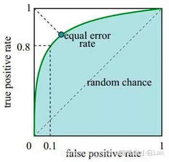
它通过 将连续变量设定出多个不同的临界值，从而计算出一系列敏感性和特异性，再以敏感性为纵坐标、（1-特异性）为横坐标绘制成曲线，曲线下面积越大，判别的准确性越高。
在ROC曲线上，最靠近坐标图左上方的点为敏感性和特异性均较高的临界值。

在医学统计里，任何一个诊断指标，都有两个最基本的特征，即敏感性和特异性。

• 所谓敏感性，就是指其在诊断疾病的时候不漏诊的机会有多大（漏诊，是真病人没有被诊断出来）；
• 所谓特异性，就是指该指标在诊断某疾病时，不误诊的机会有多大（误诊，是没病被诊断出有病了）。

单独一个指标，如果提高其诊断的敏感性，必然降低其诊断的特异性，换句话说，减少漏诊必然增加误诊，反之亦然。

所以，该指标也被引用到AI领域，用于对模型测试结果进行描述，进而反应模型的性能。

1、如何绘制ROC曲线呢

针对如何绘制ROC曲线这个问题，首先需要做一下几个步骤：

1. 根据机器学习中分类器的预测得分对样例进行排序
2. 按照顺序逐个把样本作为正例进行预测，计算出FPR和TPR
3. 分别以FPR、TPR为横纵坐标作图即可得到ROC曲线

所以，作ROC曲线时，需要先求出FPR和TPR。这两个变量的定义：

FPR = TP/(TP+FN)

TPR = TP/(TP+FP)

ROC曲线示意图如下：

综上，此时可以发现，在绘制ROC曲线中，求出FPR和TPR是重中之重。

FPR和TPR该如何计算得到呢？sklearn.metrics.roc_curve函数提供了很好的解决方案。

fpr,tpr,thresholds=sklearn.metrics.roc_curve(y_true,
                                  y_score,
                                  pos_label=None,
                                  sample_weight=None,
                                  drop_intermediate=True)

• y_true：为真值，是label
• y_score：是模型的预测结果
• 标签中认定为正的label个数，例如label= [1,2,3,4]，如果设置pos_label = 2，则认为3,4为positive，其他均为negtive

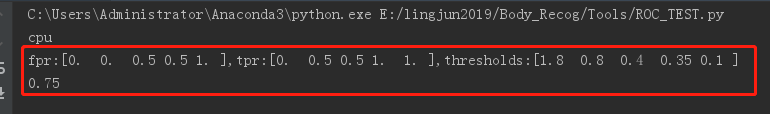
此时以下面一个案例，查看下roc_curve函数返回的数据是什么样子的：得到的就是我们所需要的FPR和TPR值，是不是很开心。

import numpy as np
from sklearn import metrics
y = np.array([1, 1, 2, 2])
scores = np.array([0.1, 0.4, 0.35, 0.8])
fpr, tpr, thresholds = metrics.roc_curve(y, scores, pos_label=2)
print("fpr:{},tpr:{},thresholds:{}".format(fpr,tpr,thresholds))

之后，我们就拿FPR和TPR数列表，来干些事情吧

import numpy as np
from sklearn import metrics
y = np.array([1, 1, 2, 2])
scores = np.array([0.1, 0.4, 0.35, 0.8])
fpr, tpr, thresholds = metrics.roc_curve(y, scores, pos_label=2)
print("fpr:{},tpr:{},thresholds:{}".format(fpr,tpr,thresholds))
roc_auc = metrics.auc(fpr, tpr)
print(roc_auc)

pyplot.plot(fpr, tpr, lw=1, label="TB vs nonTB, area=%0.2f)" % (roc_auc))

pyplot.xlim([0.00, 1.0])
pyplot.ylim([0.00, 1.0])
pyplot.xlabel("False Positive Rate")
pyplot.ylabel("True Positive Rate")
pyplot.title("ROC")
pyplot.legend(loc="lower right")
pyplot.savefig(r"./ROC.png")

最终的绘制结果是这样的（有些丑，我们接着往后看）

2、看下Dog and Cat的ROC

再回顾下上一篇文章Dog和Cat的故事：FP、FN、TP、TN、精确率(Precision)、召回率(Recall)、准确率(Accuracy)评价指标详述

这里是打印出来的AUC值和fpr，tpr，thresholds值

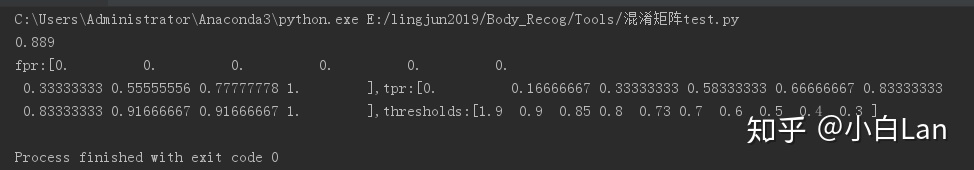
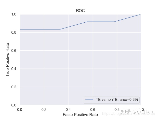
绘制的最后结果是这个样子的，是不是有一些完美了，接着往后看，我们来写实战的。

3、PyTorch来实战ROC

这里我们假定一个2分类的深度学习项目为例，如果你用过PyTorch就最好了，没用过也没关系，因为最终的形式都是要整理为规整的数据形式，之后的工作直接交给def函数来干。

def inference():
    """
    省略一大段，包括模型的加载，实例化；
    数据的加载等等，都忽略，往后看，关注数据部分
    """
    # with torch.no_grad():
    #     for idx, (input, target) in enumerate(tqdm(data)):
    #         path_raw = dataset.list_path_raw[idx]
    #         img_raw = cv2.imread(path_raw)
    #         img_raw = cv2.resize(img_raw, (1024, 1024))
    #
    #         # ---- Input and Target ----
    #         input_raw = input.to(device)
    #         Target = target.long().to(device)
    #
    #         output = model(input_raw)
    #         # ---- Outpu with Sofmax ----
    #         output_sfmx = F.softmax(output, dim=1)
    #
    #         #
    #         PD = torch.cat((PD, output_sfmx.data.cpu()), 0)
    #         GT = torch.cat((GT, Target.float().cpu()), 0)
    """
    创造标签与预测结果的数据段，分别是GT和PD
    """
    GT = torch.FloatTensor()
    PD = torch.FloatTensor()

    for i in range(130):
        pd1 =[[0.8,0.2]]
        output_pd1 = torch.FloatTensor(pd1).to(device)
        target1 = [[1.0,0.0]]
        target1 = torch.FloatTensor(target1)  # 类型转换, 将list转化为tensor, torch.FloatTensor([1,2])
        Target1 = torch.autograd.Variable(target1).long().to(device)
        GT = torch.cat((GT, Target1.float().cpu()), 0)   # 在行上进行堆叠
        PD = torch.cat((PD, output_pd1.float().cpu()), 0)

    for i in range(50):
        pd1 =[[1.0,0.0]]
        output_pd1 = torch.FloatTensor(pd1).to(device)
        target1 = [[1.0,0.0]]
        target1 = torch.FloatTensor(target1)  # 类型转换, 将list转化为tensor, torch.FloatTensor([1,2])
        Target1 = torch.autograd.Variable(target1).long().to(device)
        GT = torch.cat((GT, Target1.float().cpu()), 0)   # 在行上进行堆叠
        PD = torch.cat((PD, output_pd1.float().cpu()), 0)
    for i in range(150):
        pd1 =[[1.0,0.0]]
        output_pd1 = torch.FloatTensor(pd1).to(device)
        target1 = [[0.0,1.0]]
        target1 = torch.FloatTensor(target1)  # 类型转换, 将list转化为tensor, torch.FloatTensor([1,2])
        Target1 = torch.autograd.Variable(target1).long().to(device)
        GT = torch.cat((GT, Target1.float().cpu()), 0)   # 在行上进行堆叠
        PD = torch.cat((PD, output_pd1.float().cpu()), 0)

    confusion_matrix_roc(GT, PD, "ROC", 2)

上面的数据部分是自己创造了，我很难的好吧，为了精简的关注与ROC曲线的绘制，又要删繁就简，不能拖沓，我就自己创建一批数据吧，那就就for循环来创建吧。

• 测试数据330个，其中前130label是[1,0]，预测pd是置信率[0.8,0.2]
• 中间50个，label是[1,0]，预测pd是置信率[1.0,0.0]
• 后150个，label是[0,1]，预测pd是置信率[1,0]

将他们通过cat按行堆叠在一起，这样就把def定义的函数

confusion_matrix_roc（）

所需要的数据给准备好啦。

此时，是不是在想confusion_matrix_roc是什么？

在这里定义的，即可就亮出真身，如下：

import torch
import numpy as np
from matplotlib import pyplot
from sklearn.metrics import roc_auc_score, confusion_matrix, roc_curve, auc
def confusion_matrix_roc(GT, PD, experiment, n_class):
GT = GT.numpy()
PD = PD.numpy()
y_gt = np.argmax(GT, 1)
y_gt = np.reshape(y_gt, [-1])
y_pd = np.argmax(PD, 1) # 即行方向搜索最大值,取出元素最大值所对应的索引
y_pd = np.reshape(y_pd, [-1])
# ---- Confusion Matrix and Other Statistic Information ----
if n_class > 2:
c_matrix = confusion_matrix(y_gt, y_pd) # y_gt---标签的类别list y_pd---预测的类别list
print("Confussion Matrix:n", c_matrix)
list_cfs_mtrx = c_matrix.tolist()
print("List", type(list_cfs_mtrx[0]))
# for k in len(list_cfs_mtx):
path_confusion = r"./confusion_matrix.txt"
# np.savetxt(path_confusion, (c_matrix))
np.savetxt(path_confusion, np.reshape(list_cfs_mtrx, -1), delimiter=',', fmt='%5s')
if n_class == 2:
list_cfs_mtrx = []
tn, fp, fn, tp = confusion_matrix(y_gt, y_pd).ravel()
list_cfs_mtrx.append("TN: " + str(tn))
list_cfs_mtrx.append("FP: " + str(fp))
list_cfs_mtrx.append("FN: " + str(fn))
list_cfs_mtrx.append("TP: " + str(tp))
list_cfs_mtrx.append(" ")
list_cfs_mtrx.append("Accuracy: " + str(round((tp + tn) / (tp + fp + fn + tn), 3)))
list_cfs_mtrx.append("Sensitivity: " + str(round(tp / (tp + fn + 0.01), 3)))
list_cfs_mtrx.append("Specificity: " + str(round(1 - (fp / (fp + tn + 0.01)), 3)))
list_cfs_mtrx.append("False positive rate: " + str(round(fp / (fp + tn + 0.01), 3)))
list_cfs_mtrx.append("Positive predictive value: " + str(round(tp / (tp + fp + 0.01), 3)))
list_cfs_mtrx.append("Negative predictive value: " + str(round(tn / (fn + tn + 0.01), 3)))
path_confusion = r"./confusion_matrix.txt"
np.savetxt(path_confusion, np.reshape(list_cfs_mtrx, -1), delimiter=',', fmt='%5s')
# ---- ROC ----
pyplot.figure(1)
pyplot.figure(figsize=(6, 6))
print(PD)
fpr, tpr, thresholds = roc_curve(GT[:, 1],PD[:, 1]) # fpr, tpr, thresholds = metrics.roc_curve(y, scores, pos_label=2) 标签，分数
roc_auc = auc(fpr, tpr)
print(PD[:, 1])
pyplot.plot(fpr, tpr, lw=1, label="TB vs nonTB, area=%0.2f)" % (roc_auc))
pyplot.plot(thresholds, tpr, lw=1, label='Thr%d area=%0.2f)' % (1, roc_auc))
pyplot.plot([0, 1], [0, 1], '--', color=(0.6, 0.6, 0.6), label='Luck')
pyplot.xlim([0.00, 1.0])
pyplot.ylim([0.00, 1.0])
pyplot.xlabel("False Positive Rate")
pyplot.ylabel("True Positive Rate")
pyplot.title("ROC")
pyplot.legend(loc="lower right")
pyplot.savefig(r"./ROC.png")

认真看到这里你就会发现，其实就是我们在上一篇文章里面介绍的内容和本节中说到内容的集合，到这里，就一网打尽啦。

最后，需要用到就收藏吧，我就不信你哪天用不到。如果您觉得好，就分享给您的小伙伴，我们一起让知识的传播更高效，让技能获取更快捷，在AI的路上没有难题，只有遨游。

往期回顾

1.面试常见问题之---见招拆招

2.面试中的C++常见问题之1--10

3.FP、FN、TP、TN、精确率(Precision)、召回率(Recall)、准确率(Accuracy)评价指标详述

4.秋招简历这样写，拿offer的几率更大哦（附赠简历模板）

5.面试中的C++常见问题之11--20

小白CV将在第一时间发布CV/AI新动态，整理好文章

（最近会更加关注秋招，Good Luck）