语言abline画不出线_战胜恐惧心理：集中学习R语言的第一个小结（我的起点是：连标准误是什么都不知道）...

############ For beginners like me ##########################

# The words ahead: R is not such difficult like our imagination; 

    # just use "?" in R frequently and focus on the definition and the examples showed.

## Main Sources:

# (1) Most basic introduction of R for newcomers: https://www.youtube.com/watch?v=BvKETZ6kr9Q;

# (2) A video introducing R for begginners, 1,204,173 views

    # (entited "R Programming Tutorial - Learn the Basics of Statistical Computing"): https://www.youtube.com/watch?v=_V8eKsto3Ug&t=1022s

    # You can download the course files from https://datalab.cc/tools/r01

    # (一百万多的观看量，看一抵十，两小时的课我学了七个多小时 ); 

#(3)R files from quantitative method course of Prof. ZHAN V. Jing at the CUHK; 

    # and also the do-file of Prof. Zhan's estimable paper in 2017；

# (4) 刘思喆: 《R 常见问题解答/R frequently asked questions》;

# (5) 首都师范大学政法学院吴江老师在学术志开设的“R语言基础操作及图表制作”课程;

# (6) other useful pdf documents from R official website.

########################### Outline ####################‍‍‍‍‍

# 目录逻辑是：安装--画图--读取和保存--数据基础--数据清理--描述数据--回归模型--稳健性--深度案例

# Most basic information of R

# 1 First fancy meeting R: Installing R, RStudio, and Packages -- 安装

# 2 Graphic: plot(), Bar Charts, Histograms -- 画图

    # 彩色折线图的画法

# 3 Read & save data -- 读取和保存

    # Entering Data and Importing Data

# 4 Basis of data: data classification -- 数据基础

# 5 Data cleaning -- 数据清理

# 6 Descriptive analysis -- 描述数据

# 7 Modeling data: Regression --回归模型

# 8 Robust test -- 稳健性

# 9 A Case: Paper of Zhan2017 -- 深度案例

# Recommend other sources

######## MOST BASIC INFO. OF R ############################

# The advantages of R software. 1. Free. 2. Vector operations. 3. Great community. 4. 9000+ packages. 

    # In all, "This is R. There is no if, only how." 

# Main references in this part: 刘思喆: 《R 常见问题解答/R frequently asked questions》

# 最最基本的概念(是一切数据库的基础)：

     # row就是行(横向的)，就是case的观察个数，一般也就是n，n个observations，一般数据库中的row有成百上千。

       # 同一年观察到很多row，那就是截面数据。   

   # column就是列(纵向的)，就是变量的个数，一般也就是解释变量，即variables, 一般仅十几个，罕见过百。

## 基础性的简易文件，建议提前研读

# 官网下载中文版R建议操作卡片的地址(仅4页，基础知识，重要)：https://cran.r-project.org/doc/contrib/Liu-R-refcard.pdf

## R中的运算：

# %% 余数

# %/% 整除

# ！= 不等于

# Modulo: %% #求余数

# %>% directly jump to another line

# click run = control + enter 按“ctrl+enter“就无需用鼠标点source 中的“Run”

# equal sign are same with arrow sign. 'option + -' equals to '='

# R is not sensitive to space. In R, 'I like R' is same with 'I like             R'.

# R is not sensitive to double quote or single quote.

# R is sensitive to capital/cap.

# R begins with 1, other language begins with zero.

# 如何安装R：在搜索引擎中找R和Rstudio就能安装。this is the official place for R: https://mirrors.tuna.tsinghua.edu.cn/CRAN/

# 在R中输入一下命令，就能随机看多个漂亮的图形：demo(graphics)

log(8, 2) # 将默认底数e改为2.

# 求加权平均数

x=c(0.2, 0.3, 0.1, 0.4)

y=c(66, 77, 88, 99)

z=sum(x*y) # weighted mean

# 求小数点位数

round(3.6, 0) # 4

round(3.5, 0) # 4

round(2.5, 0) # 2 # 不是日常的四舍五入！

round(1.15, 1) # 1.1

round(1.25, 1) # 1.2

round(pi, 2) # round函数默认保留到个位数，逗号后面的数字就是设定小数点位数。

round(pi, 0)

round(12345, -2) # 结果为12300

ceiling(3.2) # 向上取整数，结果为4

floor(2.8) # 向下取整数，结果为2

###### 1 FIRST FANCY MEETING R ############################

# Video source: https://www.youtube.com/watch?v=_V8eKsto3Ug&t=1022s

# 从1：29开始，视频开始介绍较为基本的一些操作。

# Hello from Barton Poulson, the creator of this video. I'm thrilled that @freeCodeCamp.org 

  # is sharing my videos and I'm truly grateful for the appreciation that you have shown. 

  # You can download the course files from https://datalab.cc/tools/r01. 

  # You can see my other videos at https://datalab.cc. Thanks, Bart (https://bartonpoulson.com/)

# R是由新西兰奥克兰大学统计学系的 Ross Ihaka 和 Robert Gentleman 共同创立, 两人都叫R...

# 在R的官方网址上选择网站镜像 http://cran.r-project.org/mirrors.html，如 UC Berkeley下载软件副本

# 如何使用R自带的数据集

# 类似于stata，R 在 datasets 包中共提供了 102 个可以使用的数据集，用如下命令：

library(datasets)

data(USJudgeRatings)

?USJudgeRatings # see the introduction of this data set

###### Package: installing and clearing 

# pac-man: contains dplyr, tidyr, stringr, httr, ggivs, ggplot2, shiny, rio

# p_load # a function, checks to see if a package is installed, if not it attempts to install

# p_unload(dplyr, tidyr, stringr) # Clear specific packages

# p_unload (all) # Easier: clears all add-ons

# detach ("package: datasets", unload = TRUE)

.packages(all.available =TRUE) # 查看已安装的所有package

# illustrate central limit theorem 中心极限定律

par(mfrow = c(2, 2)) # A vector of the form c(nr, nc). 在Rstudio右下角Plots界面分行列展示图形

# Subsequent figures will be drawn in an nr-by-nc array on the device by columns (mfcol), or rows (mfrow), respectively.

unif

hist(unif) # 

x1

hist(x1)

x2

hist(x2) # distribution of the sample mean

x3

table(x3)

hist(x3) # distribution of the sample mean

###### 2 GRAPHIC ########################################

# pch 是 plotting character 的缩写。pch 符号可以使用 “0 : 25” 来表示 26 个标识(见刘44页文件)。

# abline() 这可以在已有图形上加一个水平线。

# 如果需要比较四个图形的区别，可将Rstudio右下角Plots区间图片呈现方式设置为：

    # par(mfrow = c(2, 2)) # A vector of the form c(nr, nc).

# 可用以下命令设置图片四周大小：

    # par(mar = c(bottom, left, top, right)) # 可设置图形边界大小

    # par(mfrow = c(1, 1)) # 这是默认状态，也就是每次以row=1，column=1的方式展示，即一次只展示一个。

# 给坐标点加入文字：plot(x, y, type="n"); text(x, y, names)

# 划一根截距为a斜率为b的线：abline(a,b)

# 画出左右底高的四边形：rect(x1, y1, x2, y2)

# 添加图例：legend(x, y, legend) 

# 用lty控制折线图中折现的形状：1: "solid", 2: "dashed", 3: "dotted", 4: "dotdash", 5: "longdash", 6: "twodash"

# 用lwd控制连线的宽度，默认值为1

# 各种颜色配比的网站(可手动配色，然后得出颜色编码)：http://colorizer.org/ (感恩吴江老师的分享)

## 先给出一个综合的例子，有点难度

#install.packages("HSAUR")

data("Forbes2000", package = "HSAUR")

attach(Forbes2000) #attach the data for R to analyze#

head(Forbes2000)

#drawing graphs

hist(marketvalue)

hist(log(marketvalue))

boxplot(marketvalue ~ category, ylab = "Market value") # category is one of the 8 columns (variables)

    # 这意味着我们不但可category这个单个变量进行boxplot，而且可对category细分类型来画箱型图。

    # 突然理解了，上述箱型图的意思是按照不同类型的category来分别画marketvalue的箱型图？

typeof(Forbes2000$category)

class(category) # factor

plot(log(marketvalue) ~ log(sales), pch = ".", main = "dv=mv") # pch='.' is better than pch = '19'

# 上述命令的另一个写法：plot(log(sales), log(marketvalue) ,pch = '.') 

abline(lm(log(marketvalue) ~ log(sales)))

##### 用ggplot2呈现更高级的图形 ############################

#install.packages("HSAUR")

data("Forbes2000", package = "HSAUR")

attach(Forbes2000) # attach the data for R to analyze

library(ggplot2)

qplot(category, marketvalue, data=Forbes2000, geom="boxplot") +

  scale_x_discrete(label=abbreviate) 

    # quickplot: qplot(mpg, wt, data = mtcars, colour = cyl)

    # scale_x_discrete(label=abbreviate) 用于解决各iv名称太长的问题***

?qplot # 认真学习此命令，对于理解R语言极有帮助，特别是学习帮助中的诸多例子。 

# 画出两个变量之间的关系

ggplot(data = Forbes2000, aes(x=log(sales), y=log(marketvalue))) +

  geom_point(color="dark green", size=0.5) +

  geom_smooth(method = "lm", se = TRUE) # 重要***

######### 查看四个变量之间两两关系：很漂亮的一系列图

#install.packages("HSAUR")

data("Forbes2000", package = "HSAUR")

attach(Forbes2000) # attach the data for R to analyze

library(ggplot2)

install.packages("psych")

library(psych)

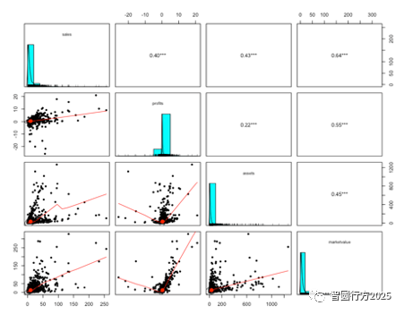
pairs.panels(Forbes2000[,c(5,6,7,8)], method = "pearson", stars = TRUE) # 重要***

?pairs.panels # 非常好用的一个函数。

    # 记住pairs.panels；ci= TRUE是指按照95%置信区间来计算相关性

↓：用pairs.panels画出来的就是下面这个图

# 通过log将弯曲度大的变量扶正/normalize highly skewed variable

lgsales

lgassets

lgmarketvalue

# 多元回归 Run multiple linear regression on marketvalue

reg

summary(reg)

### 2.1 plot is the basic one. 

# easy beginning

x2

e

names(e) = letters [1:10] # use letters to name for values 

e # can see the name of each value

names(e) # "a" "b" "c" "d" "e" "f" "g" "h" "i" "j" NA 

y2

plot(x2,y2, pch = 19, col= "red") # to see solid dot and red color

boxplot(x2,y2, pch = 19, col= "red", main = "boxplot", xlab="x2", ylab="y2") # to see boxplot

boxplot(y2~x2, pch = ".", col= "red", main = "boxplot", xlab="x2", ylab="y2") # ?

##eg for iris with 150 cases and 5 variables

# 调用系统内数据

library (datasets)

head(iris)

# 画图

boxplot(iris$Sepal.Length, iris$Sepal.Width, iris$Petal.Length, xlab="IV", ylab="values of IV", main="Boxplot")

plot(iris$Sepal.Length, iris$Sepal.Width, col="#cc0000", pch=19, main ="title", xlab="x title", ylab="y title") # 生成两个变量的散点图，plot(x,y).

# Formula plot with options

plot(exp,1,5)

plot(dnorm, -3, +3,

     col = "#cc0000",

     lwd = 1, # thinner line

     pch = 21:25, # 19: solid circle; 21: filled square

     main = "Standard Normal Distribution",

     xlab= "z-scores",

     ylab= "Desity")

## Another example for plot 

#This challenge is about famous houses in the pretty town of Brigadoon

distances=c(51,65,175,196,197,125,10,56)#distances of 8 houses from the town centre in m

bearings=c(10,8,210,25,74,12